I have been conscious for a long time that, on a clear day, the view from Dunbar includes mountains that are a long way to the north. But I never knew which mountains they were, exactly. It was clear a day or two ago, so, while out on my permitted exercise, I set my camera to maximum zoom and took a panoramic sequence of photos of the horizon.
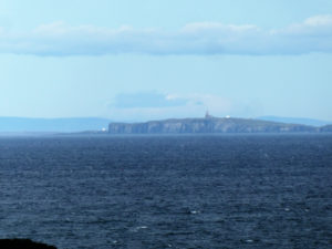
In this example, the nearest land, with the grey lighthouse and little white towers, is the Isle of May, out in the mouth of the Firth of Forth. The sliver of low land to its left is the Fife coast on the North side of the firth. Behind them are distant mountains in the Highlands, but which bit of those is which?
In an attempt to find out, I made use of the fact that, as a University employee I have access to Ordnance Survey maps of all of Britain via Edina Digimap. This web site allows a subscriber to zoom right in to any spot, place the cursor onto the map, and to read off the National Grid co-ordinates of that spot. I did this for the spot from where I took the photographs, and for a variety of landmarks, towns, and mountains in Fife, and beyond that in the Highlands, giving me a list like this:
easting  northing  name
368320 678550      Bench
365500 699364      May_light
365083 699950      May_NW
365962 698827      May_SE
#364118 709886      Fife_Ness
361284 708525      Crail_town_centre
357597 709471      Kellie_Law
The bench is the spot from where I took the photographs. (Locals: it is the bench inset into the wall on Queen’s Road, opposite the sheltered flats, a little bit east of the parish Church.) With this, it is straightforward to calculate the distance to each landmark from Pythagoras’s theorem and the compass bearing using trigonometry. I show the code below, but it is too long to break up the text with it. The code also draws a vertical line for each landmark, adding its name and distance, all ready for comparison with the photos.
The next thing I did was to glue the individual photographs into a panorama. I used hugin for this. Hugin is excellent and I used to use it a lot; I have used it a lot less since I got a camera with a built-in panorama mode. But the camera does not buy the idea that you might want to do a panorama with the zoom lens at anything except the widest angle, so I had to resort to hugin for this job. Having produced the panorama, I loaded it into gimp as the base layer, and loaded the picture drawn by my code into a separate layer. I then stretched the layer with the markers until it matched the landmarks which I could identify on both the photographs and the map. These were the three towers on the Isle of May, and the three large wind turbines (marked WT) that I could see on the Fife coast. The end result looks like this:

Whether you can see the markers depends on what sort of device you are trying to read this on — they are readable on the image I uploaded to the WordPress server but don’t seem to be large enough in the final web page. You may want to download the moderate resolution version (0.5 Mb) or the full version (10 Mb). To give an idea of what the whole thing looks like, here is a section of it.
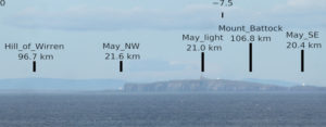
The furthest mountains that can be seen are in the south and east of the Cairngorms: Mount Battock is 14 km south of Aboyne, Mount Keen is 10 km south of Ballater and Lochnagar is 10 km south of Balmoral Castle. One thing you can not see from this particular viewpoint is the lighthouse on Fife Ness. It is almost exactly behind the one on the Isle of May; I commented it out of the data file so that its label did not make the plot more cluttered.
Postscript: here is the python code
#!/usr/bin/python3

import numpy as np
import matplotlib.pyplot as plt

## Read the co-ordinates from the data file
xydat=np.genfromtxt("coords.dat",skip_header=1,usecols=(0,1))
## Read the landmark names
names=np.genfromtxt("coords.dat",skip_header=1,usecols=(2),dtype="str")


### Loop over the landmarks, calculating the bearings and distances
### of each landmark from the photographer
dims=xydat.shape
npts=dims[0]
bearings=np.zeros(npts)
ranges=np.zeros(npts)
for i in range(1,npts):
    dx=xydat[i,0]-xydat[0,0]
    dy=xydat[i,1]-xydat[0,1]
    bearings[i]=(180/np.pi)*np.arctan2(dx,dy)
    ranges[i]=np.sqrt(dx*dx+dy*dy)/1000
    print(i,format(bearings[i],'6.4f'),
          format(ranges[i],'6.4f'),
          format(bearings[i]-bearings[1],'6.5f'),names[i])

## Print out the bearings and landmark names in clockwise order
ix=np.argsort(bearings)
for i in range(0,npts):
    j=ix[i]
    print(format(bearings[j],'6.4f'),
          format(bearings[j]-bearings[1],'6.5f'),
          names[j])

## Make a plot to overlay on the final image
plt.ion()
plt.close("all")
plt.rcParams.update({'font.size': 5}) ## Font is a lot smaller than default
fig=plt.figure(1,figsize=(20,0.7)) ## Figure is very long and thin
ax=plt.axes(frameon=False) ## Turn off usual axes
###ax=plt.axes()

## Parameters for vertical lines. They are of random heights so the text
## of neighbouring landmarks are less likely to clash
tops=np.random.rand(npts)*1.4
llen=0.1
xlim=[-27,-6]

## Draw each vertical line and write its text. If it is outwith the desired
## range we don't draw it at all
for i in range(1,npts):
    if (bearings[i] > xlim[0])*(bearings[i] < xlim[1]):
        ax.plot(np.array([1,1])*bearings[i],[0,llen+tops[i]],"k-")
        ax.text(bearings[i],llen+tops[i]+0.45,names[i],
                 horizontalalignment='center')
        ax.text(bearings[i],llen+tops[i]+0.1,format(ranges[i],'5.1f')+" km",
                 horizontalalignment='center')

## Tidy plot and write it out.
ax.yaxis.set_visible(False)
ax.xaxis.set_visible(True)
## ax.set_frame_on("False")
ax.set_xlim(xlim)
ax.set_ylim([-0.2,1.8])
ax.xaxis.set_ticks_position('top')
plt.savefig("graticule.png",bbox_inches="tight",dpi=1400,transparent="True")

