Guess what: we are on strike. Again. This time, our employers have at last decided to negotiate, and there are rumours emerging of actual progress in those negotiations. While on strike I have done a long series of overdue domestic tasks, the last of which was admitting the man from EDF to replace our traditional electricity and gas meters with shiny new smart meters. These refused to work because they cannot connect to their network from our house, exactly as the installer predicted. I will have to continue reading them myself or letting a person in to do it; the only advantage is that I will no longer receive incessant pestering phonecalls from EDF’s call centre.
I had heard nasty rumours of billing trouble where smart meters fail to work in smart mode. To get my ducks in line for any forthcoming battle I typed the data from my gas / electricity bills into the computer and plotted them up using python. I went back to 2004; before then I was getting gas and electricity from different suppliers with different reading dates.
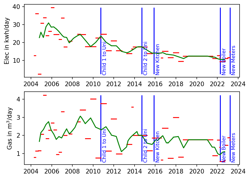
The original data are the horizontal red lines. Each bill includes data for the current and previous meter reading; I cannot tell the detail of what happened during the billing period so I have to assume that the consumption rate is constant between one meter reading and the next.
It was quite hard to infer any long-term changes by eye, especially for the 2004-2008 period, when the bills came every three months rather than every six months. There is also a chunk of missing data between 2019 and 2021 — this is because EDF remove your bills from their web site after three years. (If I had realised this I would have downloaded and kept them.) For this reason, I joined the flat red lines up into a continuous time series, interpolated it to every day, and calculated a 365-day running mean (green line).
The electricity usage shows a steady decline over the last two decades, visible to the eye even without the running mean. I suspect that this is from a combination of reasons: decrease in the number of people in the house from four to two, improved energy efficiency of modern electronic gear (including lightbulbs), the change from a traditional to an induction hob in 2016, fiery death and non-replacement of a tumble-drier, etc. No individual event appears to cause a step change, though.
There does also appear to be a decrease in gas usage, but it is far from obvious how significant it is. It does not seem to have decreased to half its previous value in line with the occupancy of the house. The interesting question is whether the switch from a non-condensing to a condensing boiler in 2022 will prove to have made a noticeable difference; I shall have to wait a couple of years to get anything approaching an answer.
Code postscript
The data file looks like this:
date1,date2,prevelec,elec,prevgas,gas,prevcode,code
## O=official read, C=Customer Read, E=Estimate
2004-04-26,2004-06-17,85287,85950,9712,9753,C,E
2004-06-18,2004-09-13,85950,89094,9753,9853,E,E
2004-09-14,2004-12-13,89094,89317,9853,9957,E,O
## Bad elec estimate 10319 in these next two lines replaced with 05000
2004-12-14,2005-03-16,02174,05000,9957,0148,O,E
2005-03-17,2005-06-15,05000,08049,0148,0528,E,O
And the code that produces the plot is as follows:
#Plot gas/electricity meter data

import matplotlib as mp
mp.use("Qt5Agg")

import numpy as np
import matplotlib.pyplot as plt

## Events to mark on plot.
evdates=np.array(["2010-09-30","2014-09-14","2015-11-15", "2022-04-15",
                  "2023-03-20"],dtype=np.datetime64)
events=np.array(["Child 1 to Uni","Child 2 to Uni","New Kitchen",
                 "New Boiler","New Meters"])

## Read in the ASCII fields (including the dates)
strs=np.genfromtxt("gaselec.dat",delimiter=",",usecols=(0,1,6,7),dtype="str",
                   skip_header=1)
## Read in the numeric fields
dat=np.genfromtxt("gaselec.dat",delimiter=",",usecols=(2,3,4,5),skip_header=1)

## Convert dates to Numpy's datetime64 format
sdate=np.array(strs[:,0],dtype=np.datetime64)
edate=np.array(strs[:,1],dtype=np.datetime64)

## Number of days in each billing period
days=np.array(edate-sdate,dtype=np.float64)

### Fix meter rollovers by adding 10000 (gas)
## or 100000 (elec) to the second reading
igr=np.where(dat[:,3] < dat[:,2])[0]
dat[igr,3]=dat[igr,3]+10000
ier=np.where(dat[:,1] < dat[:,0])[0] if len(ier) > 0 :
    dat[ier,1]=dat[ier,1]+100000

## Units used in each billing period
gasuse=dat[:,3]-dat[:,2]
elecuse=dat[:,1]-dat[:,0]
## Units per day in each billing period
gaspd=gasuse/days
elecpd=elecuse/days
nbills=len(sdate)

## Construct daily time series, and then smooth it with a year-long boxcar
dates1d=np.arange(sdate[0],edate[-1],1)
ndays=len(dates1d)
stepdates=np.zeros(nbills*2,'datetime64[D]')
stepepd=np.zeros(nbills*2)
stepdates[0::2]=sdate
stepdates[1::2]=edate
stepgpd=np.zeros(nbills*2)

stepepd[0::2]=elecpd
stepepd[1::2]=elecpd
stepgpd[0::2]=gaspd
stepgpd[1::2]=gaspd

epd1d=np.interp(np.int32(dates1d),np.int32(stepdates),stepepd)
gpd1d=np.interp(np.int32(dates1d),np.int32(stepdates),stepgpd)
kernel=np.ones(365)
epdra=np.convolve(epd1d,kernel,mode="valid")/365
gpdra=np.convolve(gpd1d,kernel,mode="valid")/365

## Plotting starts here
plt.ion()
fig,(ax1,ax2)=plt.subplots(2,1,num=2,clear=True)
labsize="small"
offset=50
## Plot for electricity
for i in range(0,nbills):
    ax1.plot((sdate[i],edate[i]),elecpd[i]*np.array([1,1]),"r-")
ax1.set_ylabel("Elec in kwh/day")
ax1.vlines(evdates,np.min(elecpd),np.max(elecpd),color="blue")
#ax1.plot(stepdates,stepepd,"g-",linewidth=1)
#ax1.plot(dates1d,epd1d,"k.")
ax1.plot(dates1d[(364//2):(len(epdra)+364//2)],epdra,"g-")

for i in range(0,len(evdates)):
    ax1.text(evdates[i]+offset,np.min(elecpd),events[i],color="blue",
             rotation="vertical",size=labsize)
## plot for gas
for i in range(0,nbills):
    ax2.plot((sdate[i],edate[i]),gaspd[i]*np.array([1,1]),"r-")
ax2.set_ylabel("Gas in m$^3$/day")
ax2.vlines(evdates,np.min(gaspd),np.max(gaspd),color="blue")
for i in range(0,len(evdates)):
    ax2.text(evdates[i]+offset,np.min(gaspd),events[i],color="blue",
             rotation="vertical",size=labsize)
ax2.plot(dates1d[(364//2):(len(gpdra)+364//2)],gpdra,"g-")


plt.savefig("powerusage.png",dpi=150,bbox_inches="tight")