Despite my efforts to ensure that I understood it, we never got to use the ERT gear during the spring of 2021. However, it currently appears that we are going to be able to travel to Shropshire for this year’s geophysics field trip (see many previous blog posts). Unfortunately, our colleagues from France and Germany can not travel to the UK, so, in addition to the gravity and seismics that we usually contribute to the trip, we need to also supply as many other techniques as we can dust off. The ERT gear will definitely go, and we now also have magnetometry.
The School of GeoSciences has had proton-precession magnetometers for a while. They consist of a box of electronics and a sensor consisting of a plastic cylinder with a coil of wire in its walls, filled with kerosene. However, a colleague recently realised that all of the electronics boxes had suffered some form of electronic death, and ordered some more. The new boxes come with a GPS unit so that you know where your measurements were taken. Before taking any of this gear on the trip I thought I had better make sure that it works, and that I and the other staff going on the trip knew how to operate it.
After a few basic tests on the grass outside the geology building I rounded up some assistants and took the gear to an open space on Blackford Hill. Here, we laid out a grid of points at a spacing of 5m. The grid was 50m long and 25m wide; we could not make it wider without walking through some impenetrable shrubs.
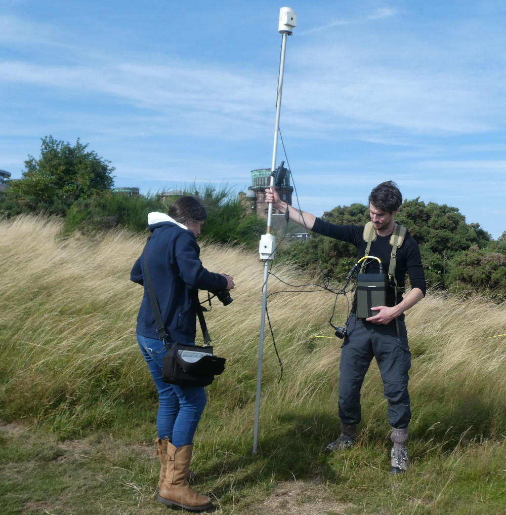
The photo shows Ph.D student David with the electronics box strapped to his chest. The white cans on the pole are two separate sensors; the GPS unit is on the pole between the sensors, just above David’s hand. We are using two sensors so that we get an estimate not only of the magnetic field, but also of its vertical gradient. You can also get a sense from the photo of how thick the grass was and how windy it was: both of these factors made it a bit difficult to use our 50m tape measures to lay out an accurate grid. To take the data the operator simply walks to each grid point in turn, presses the “Cycle” button at each location, and holds the staff still until the electronic box has taken one measurement with each of the two sensors.
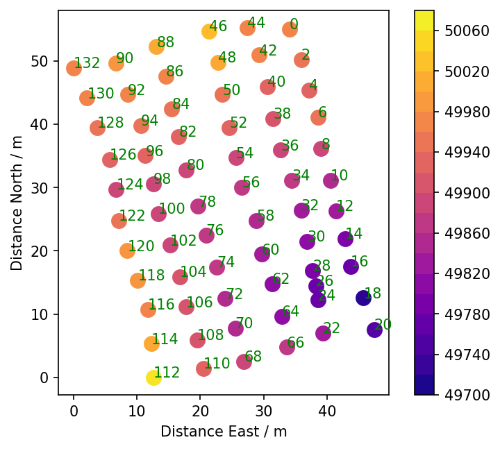
The above plot shows the relative positions of the data points; the colours show the magnetic field strength from the upper sensor in nT (nanoTeslas). It is clear that the GPS is precise enough to use for a 5m grid if you are away from trees. (I have also demonstrated, using a grassy area on the Kings Buildings campus, that it is NOT precise enough for a 2m grid under trees.) I have added the station number to each dot — they are all even numbers because each sensor gets its own station number. It is clear from the numbers that station 26 was caused by the operator taking an extra reading rather than because the GPS reported an erroneous location. The fact that the data change smoothly across the grid suggests that the variation is real, and is not just noise in the sensor. To investigate this a little further, I plotted the data from the two sensors and the difference between the sensors. 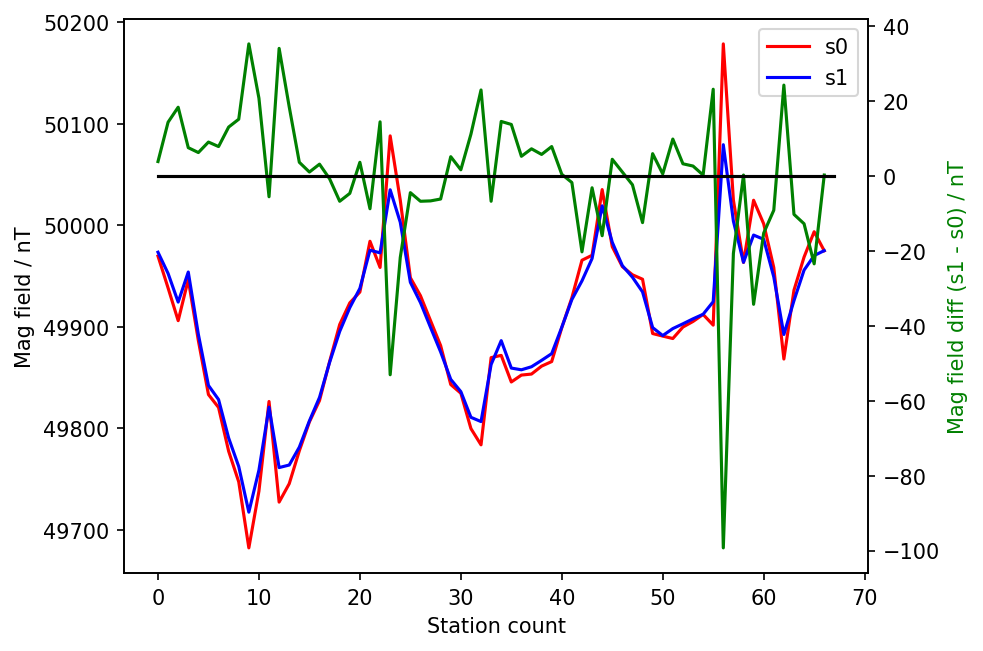
This is all very hopeful. The two sensors are recording almost the same field as each other, and the difference between the sensors is negatively correlated with the average of the two sensors.
In addition to the dual sensor rig I have already described we had a second electronics box with a single sensor. I propped this up in a gorse bush and left it logging continuously to provide a correction for any time variation in the Earth’s magnetic field. The data from it looked mostly like noise, so I concluded that the sensor was not working properly. I shall have to check whether it has sufficient kerosene in it, and whether any of the other, older, sensors that we have work any better.