It was nice to spend a day working at the University, shortly before it closed down for Christmas. The reason I dragged myself in was that, as partial recompense for missing the field trip, we hope to give the 4th-years a couple of days in the field during the reading week in the middle of the spring semester. Normally, when we go on the field trip we provide gravity and seismic surveying, relying on our colleagues from the Universities of Münster and Paris-Saclay to provide other techniques. To provide a usefully broad experience in reading week, we would have to provide at least some of those techniques ourselves. This meant a serious rummage in the storage area and the exhumation of some kit that has been used only rarely, if at all, in recent years.
Magnetic surveying should have been straightforward as we have several proton-precession magnetometers. There is not much to go wrong with the sensors themselves: they are just cylinders with a coil of wire built in, filled with kerosene. Unfortunately, the electronic control boxes that make the sensors work were another matter: we had several, but they all appeared to have suffered some sort of electronic death. Some more had been ordered, but after getting them out of the packing and fitting the batteries, we realised we needed an extra cable to connect them to a computer. Checking the magnetometers out properly is still on the “to do” list.
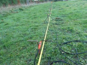
We got further with the electrical resistivity tomography (ERT) gear. The gear itself is quite old, but whatever computer used to control it has been replaced with a raspberry pi which runs the original software in an emulator. To make a measurement, the 25 electrodes are pushed into the ground with equal spacing and connected to a special cable. The cable connects to the main control box which itself is connected up to the raspberry pi.

The control software can then be instructed to do some checks to ensure that all electrodes are making good contact, and then to make a set of measurements. The configuration file we used performs a Wenner array measurement for all possible sets of four equally-spaced electrodes in the array, pushing a current, I, through the outer two electrodes and measuring the voltage, V, between the two inner electrodes. If the ground has a uniform resistivity, ρ, then it can be calculated from the measurements as ρ = 2 π a V / I, where a is the spacing between adjacent electrodes. In real life, ρ varies from place to place; this type of survey is done to find out how it varies.
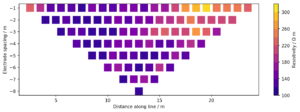
Our survey with 25 electrodes has 92 different sets of four equally spaced electrodes. The control software takes several minutes to make all 92 measurements, presenting you at the end with a file containing 92 values of V/I and the electrode positions for each. Even though the resistivity is not uniform, we calculate 2 π a V / I anyway and call it the apparent resistivity. We can start looking at the apparent resistivity values just by plotting them out, with each different spacing in a different row.

This kind of plot is called a pseudosection. We can already see from it that there is a region of higher resistivity at the right-hand end of the line, near the surface. For proper interpretation we need to estimate from the apparent resistivities how the actual resistivity varies with position. This is a tricky inverse problem, and there are a variety of software packages available to carry it out.
The best known such program is a commercial package called RES2DINV (available from its suppliers). We had a license for this in the distant past but have long ago lost the “dongle” which tells your computer that you have a right to use the software. I had to re-download the software and run it in free demo mode, which restricts the user to 84 electrodes (not a problem when I only had 25) and 4 iterations (which I had to hope was enough). RES2DINV’s initial attempt at an inversion looks like this:

I clearly have some learning to do when it comes to getting the best out of this program, if only to make the labels a readable size.
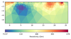
RES2DINV has competition these days from BERT (http://resistivity.net/bert/), which has the great advantage of being Free Software. Unlike RES2DINV, which is delivered as a Windows binary, BERT is at least partly written in python and is most easily installed in an Anaconda or miniconda environment. I learned enough about this to get it going, and then had to do some coding to convert the data that comes out of the ERT gear into a form that BERT would ingest. After a bit of tinkering, my end result looks like this:

BERT and RES2DINV are in agreement that there is an area of higher resistivity on the right and of lower resistivity on the left. They also agree that the lower-resistivity area is at a greater depth. To do a better job of comparing them I need to work out how to get them to use better-matched colour scales.
Many thanks are due to several colleagues who helped me to set the gear up and to take it down afterwards.

