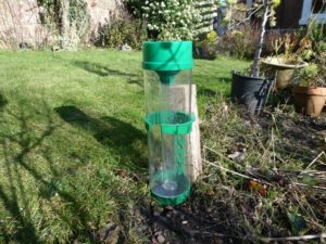
One of my birthday presents last year was a proper, official-shaped rain gauge. It took me a while to get around to setting it up, mostly because of the difficulty of picking a good spot in the garden: almost everywhere is close to a wall, under a tree, or is a place where a rain gauge would be a trip hazard. I eventually set it up in a flower bed, with a stout post whacked into the ground to hold it vertical.

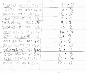
Having set it up, I had to start reading it, of course. You are really supposed to read rain gauges every day at 09:00GMT, but there was fat chance of that happening. During the working week (except while I am on strike) I am at work by 09:00, and I have a terrible memory anyway. The best thing I could think of to do is to read it when I remember and to record the exact time at which I read it. So the raw data looks like this:

Each reading has a date, a time, and a rain reading in mm — this is the rain that fell between the current date and the date on the previous line. Clearly I was not going to be satisfied with leaving the data in a notebook: it had to be entered into the computer and plotted. It helps that the dates in the notebook are in one of the commonest variants of the ISO standard. Once typed up, the last bit of the data file is:

2020-03-01T08:40 6.1
2020-03-02T08:58 1.8
2020-03-03T11:11 0.4
2020-03-04T14:21 0.0

…so there are two columns separated by a space, with the date and time forming a single item in the first column. My first cut at plotting the data using python and matplotlib went as follows:

#!/usr/bin/python3

## Code to plot rain gauge data. Data are in two columns: time in ISO
## format and rainfall in mm. The rainfall is that which occurred in
## the time between the timestamp on its own line and the timestamp on
## the previous line.

import numpy as np
import matplotlib.pyplot as plt

## Read the file in as strings
dat=np.genfromtxt("rain.dat",dtype="str")

## convert the RH colum (rain) to floating-point numbers
rain=np.float64(dat[:,1])

## Convert the LH column to datetime64 data type. We get units of
## minutes based on the data. It would be preferable to be able to
## force this.
date=np.array(dat[:,0],dtype=np.datetime64)

### time step between measurements in days
timestep = np.array((date[1:] - date[0:-1]),dtype=np.float64)/(24*60)

rrmmd = rain[1:] / timestep ## #rain rate in mm/day

rrmmd=np.concatenate(([0],rrmmd))

## Clear up windows and set up plot
plt.ion()
plt.close('all')
fig,ax=plt.subplots(1)

## Plot the data as a step plot
ax.step(date,rrmmd,where="pre")

plt.ylabel("Rain rate / mm per day")
plt.axhline(0,linestyle="dashed",color="black")

## This does the Right Thing with axis labels that are dates, without
## you having to fiddle with it yourself.
fig.autofmt_xdate()

plt.savefig("rain.png",bbox_inches="tight")

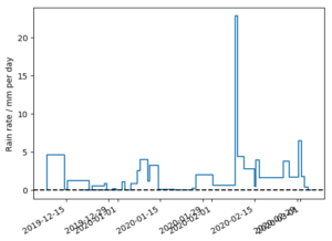
Note that we use numpy’s datetime64 data type for the times. Time is the messiest of all co-ordinates to plot against on account of our fondness for seeing it in terms of days, months and years: all awkward and non-constant multiples of each other. The datetime64 data type tames this problem somewhat, and matplotlib is happy to use the data type and to label the time axis appropriately without the user having to do anything special. There is little point plotting the actual rain readings as each reading was taken over a different length of time. Instead, I have divided the readings by the time differences between readings to give rain rates in mm/day. The result comes out like this:

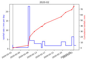
It is progress, but it will clearly not do once I have a few years’ worth of data. As meteorologists are fond of thinking of rain in terms of months, I decided to make separate plots of each month. Some more use of the datetime64 datatype allowed me to set up markers at the end of each month (actually at the official gauge-reading time of 09:00 the following day). I also calculated the cumulative rainfall for the month, correcting it as far as possible to give the total between 09:00 on the first day of successive months. The code got too long to post here, but the result for February is like this:

The February total of 75.2mm is a lot more than the climatological mean of 40mm — this fits nicely with the fact that 2020 had the second wettest February on record in Scotland.

Postscript:

I added a line to the code so that every time I run it, it uploads updated plots to the web for for the current month, the previous month, and the month before that.

Gauging the Rain / Hugh's Geophysical Blog by blogadmin is licensed under a Creative Commons Attribution CC BY 3.0