In this post, I thought I would show you how to load some time series data into a Pandas DataFrame.

The obvious choice of data is the School of GeoScience’s weather station, archive data is available for it on the web. The met station is positioned on the top of JCMB which has the view in the banner above 🙂

You can find the accompanying Jupyter Notebook here which contains runnable code and a more complete description.

1 Loading the weather station data to a Pandas DataFrame

The data is archived both in monthly snapshots and annual compilations – we will work with the latter.

The files are stored either as monthly or annual data. for example:

• Annual filenames: http://xweb.geos.ed.ac.uk/~weather/jcmb_ws/JCMB_2007.csv
• Monthly filenames: http://xweb.geos.ed.ac.uk/~weather/jcmb_ws/JCMB_2007_Nov.csv

If you look at one of the annual files, you can see:

• The top line of the file has column names
• The entries are comma separated
• The first column is date-time information
• The other columns all contain floats

Because of the mix of data types, we will need to use a Pandas DataFrame.

We want to create a single data frame which contains the met data for the years 2011-2014 inclusive, but the data is stored in separate files for each year. To do this, we use a loop to load each annual file into a data frame and then we append it to a data frame that will contain the whole sequence, which we call df_full.

df_full = pd.DataFrame()

years = [2011, 2012, 2013, 2014]

for year in years:
    url = "https://www.geos.ed.ac.uk/~weather/jcmb_ws/JCMB_"+str(year)+".csv"
    df_tmp = pd.read_csv(url)
    df_full = df_full.append(df_tmp)

Let’s have a quick look at some of the features of this the DataFrame.

1.1 We can find the number of rows and columns using:

df_fill.shape

Tells us that there are 8 columns and 2,081,999 rows. This is quite a lot of data.

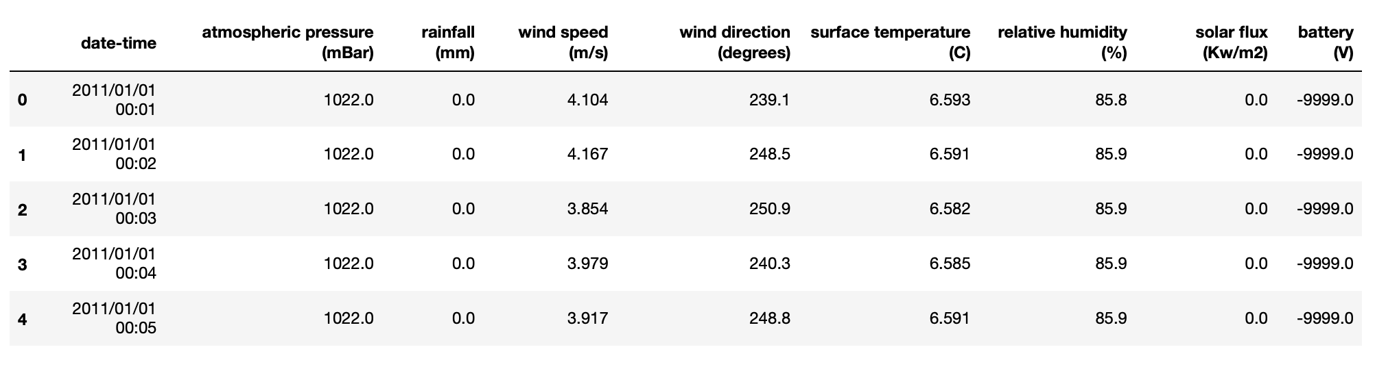
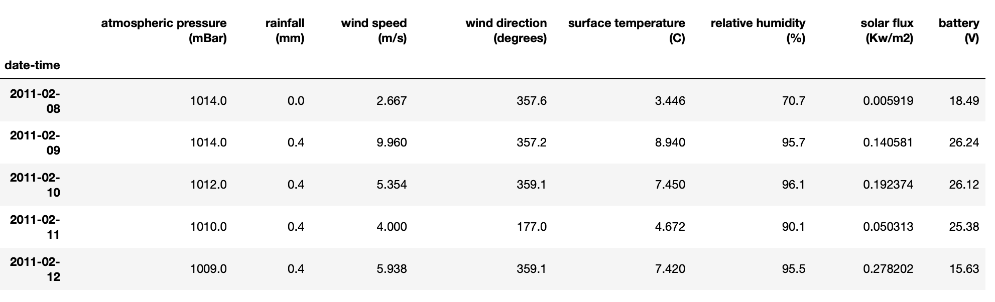
1.2 To see the top few lines of the DataFrame:

By running the head() method on the data frame we can see that there are so many rows because the data is sampled every minute. We can also see the different types of data stored in the data frame including temperature, pressure and windspeed information. Also note that we have a date-time column that we want to index the data by (i.e. instead of having the integer numbers in the leftmost column, we want date times – this allows for easier processing of the time series as we will see in section 3)

df_full.head()

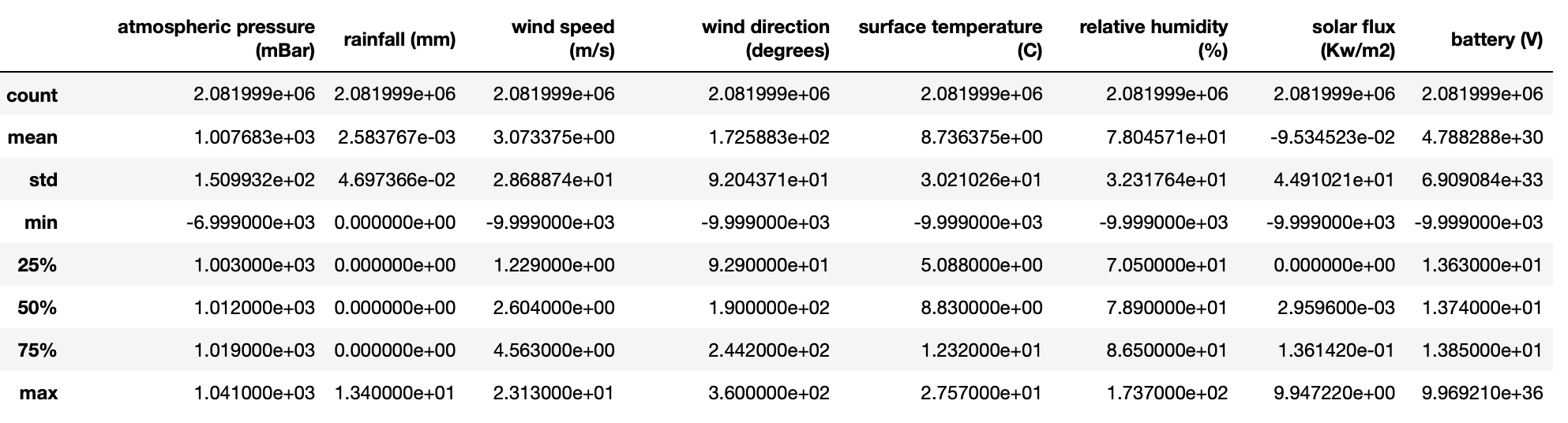
1.3 To get summary statistics of each column:

The describe method is really useful at summarising what is in each column. It also highlights potential problems with a dataset that need cleaning. In the example below, have a look at the min row. The minimum value in many columns is either -9999.0 or -6999.0. This will be the default value recorded when the sensor has not measured it correctly. We will need to filter these out.

df_full.describe()

2 Cleaning the data

The quick look at the data above highlights two thing we need to fix:

1. The describe method highlighted that there are the values -9999.0 and -6999.0 in the dataset. Whilst I have not checked whilst these are there, I suspect that these are the default values saved when the sensors have not recorded properly. These will need to be removed, we will cover them to NaNs
2. The data-time column a series of strings which we will want to convert to a date-time object and then use that as the index.

2.1 Removing the spurious values

To convert the entries with values -9999.0 and -6999.0 to NaNs is easy:

df_full = df_full.replace(-9999.0,np.NaN)
df_full = df_full.replace(-6999.0,np.NaN)

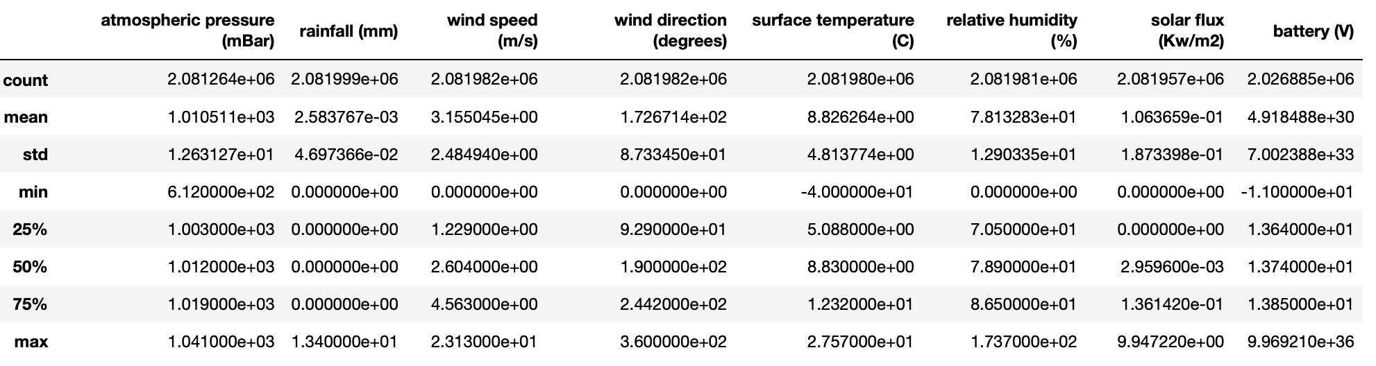
We can check this has worked by by re-running `df_full.describe()`

2.2 Setting the index to be the date-time

The first thing I tried was:

df_full['date-time'] = pd.to_datetime(df_full['date-time'], format='%Y/%m/%d %H:%M')

But this threw the error

ValueError: time data 2011/01/01 24:00 doesn't match format specified

I assume that this is because the definition of the 24 hour clock in Python does not actually include 24:00

So, to deal with this I coerce the conversion to datatime to return a NaNs whenever it fails so that I can just remove these entries:

df_full['date-time'] = pd.to_datetime(df_full['date-time'], format='%Y/%m/%d %H:%M', errors='coerce')
df_full = df_full.dropna()

The date-time column now contains date-time objects. All that I need to do now is set the index to be the date-time and check that this has worked using the head method:

df_full = df_full.set_index('date-time')
df_full.head()

3. Plotting and subsetting the time series

I am not going to do any analysis of the data in this post, just show you how to plot and resample the time series.

3.1 Plotting all the data

Since we have this data inside a DataFrame, and we have set the index to be a Date-Time object – Pandas will do most of the work for formatting the date-times on the x-axis.

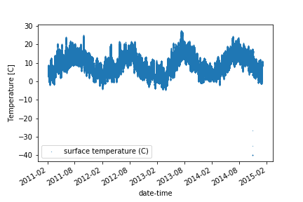
For example, we can simply plot all the data in the temperature column. The data looks quite noise because it was measured every minute!

df_full.plot(y='surface temperature (C)', style='.', markersize=0.5)

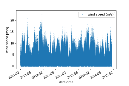
And similarly for windspeed:

df_full.plot(y='wind speed (m/s)', style='.', markersize=0.5)

3.2 Extracting subsets based on the date-time

The use of date-times as an index also makes it trivial to select subsets of the data based on time slices.

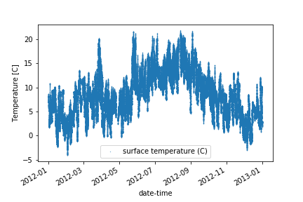
For example, to extract a and plot single year:

df_full['2012'].plot(y='surface temperature (C)', style='.', markersize=0.5)

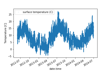
And to extract and plot an arbitrary date range:

df_full['2012-06':'2014-06'].plot(y='surface temperature (C)', style='.', markersize=0.5)

3.3 Resampling the data at daily intervals

If you look back at any of the head() calls above, you will see that the data is recorded at minute intervals and that this means we are working with over 4 million rows.

• One approach to reduce the size of the data is to remove the daily cycles by resampling at daily intervals.
• This is easy now we have the data stored as a time series:

dailyResampling_max = df_full.resample('D').max()
dailyResampling_median = df_full.resample('D').median() 
dailyResampling_min = df_full.resample('D').min()

The example above extracts the max, min and median values that occur each day for each column.

dailyResampling_max.head()

Notice that the time intervals in the index column on the left are now daily.

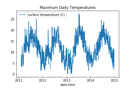
Let’s plot the temperature data resampled at daily intervals. If you compare it with the plot above, you can see that there is significantly less scatter because we have removed the daily cycles.

• The Maximum values, presumably in the day time, are very clean and range from 0 to 27 ish.
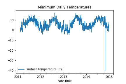
• The Minimum values are typically less than 12 degrees and it looks like there is one spurious point at -40 degrees.

4. Summary

In this post I have show you how to load, clean, plot and resample weather station data.

In future posts, I’ll show you how to analyse and forecast from this data.

Working with the Edinburgh University Met Station Data in Python / Mark Naylor’s Blog by blogadmin is licensed under a Creative Commons Attribution CC BY 3.0

Share