The second-order structure function corrected for systematic error.

The second-order structure function corrected for systematic error.

In last week’s post, we discussed the corrections to the third-order structure function $S_3(r)$ arising from forcing and viscous effects, as established by McComb et al [1]. This week we return to that reference in order to consider the effect of systematic error on the second-order structure function, $S_2(r)$ . We begin with some general definitions.

The longitudinal structure function of order $n$ is defined by:

(1) $\begin{equation*} S_n(r) = \left\langle \delta u^n_L(r) \right\rangle, \end{equation*}$

where $\delta u_L(r)$ is the longitudinal velocity difference over a distance $r$ . From purely dimensional arguments we may write:

(2) $\begin{equation*} S_n(r) = C_n \varepsilon^{n/3}\,r^{n/3}, \end{equation*}$

where the $C_n$ are dimensionless constants.
However, as is well known, measured values imply $S_n(r)\sim \, r^{\zeta_n}$ where the exponents $\zeta_n$ are not equal to the dimensional result, with the one exception: $\zeta_3 = 1$ . In fact it is found that $\Delta_n = |n/3 - \zeta_n|$ is nonzero and increases with order $n$ .

It is worth pausing to consider a question. Does this imply that the measurements give $S_n(r)=C_n \varepsilon^{\zeta_n}r^{\zeta_n}$ ? No, it doesn’t. Not only would this give the wrong dimensions but, more importantly, the time dimension is controlled entirely by the dissipation rate. Accordingly, we must have: $S_n(r)=C_n \varepsilon^{n/3}r^{\zeta_n}\mathcal{L}^{n/3-\zeta_n}$ , where $\mathcal{L}$ is some length scale. Unfortunately for aficionados of intermittency corrections (aka anomalous exponents), the only candidate for this is the size of the system (e.g. $\mathcal{L} = L_{box}$ ), which leads to unphysical results.

Returning to our main theme, the obvious way of measuring the exponent $\zeta_n$ is to make a log-log plot of $S_n$ against $r$ , and determine the local slope:

(3) $\begin{equation*} \zeta_n(r) = d\,\log \,S_n(r)/d\, \log \,r.\end{equation*}$

Then the presence of a plateau would indicate a constant exponent and hence a scaling region. In practice, however, this method has problems. Indeed workers in the field argue that a Taylor-Reynolds number of greater than $R_{\lambda}\sim 500$ is needed for this to work, and of course this is a very high Reynolds number.

A popular way of overcoming this difficulty is the method of extended scale-similarity (or ESS), which relies on the fact that $S_3$ scales with $\zeta_3 =1$ in the inertial range, indicating that one might replace $r$ by $S_3$ as the independent variable, thus:

(4) $\begin{equation*}S_n(r) \sim [S_3(r)]^{\zeta_n^{\ast}},\qquad \mbox{where} \qquad \zeta_n^{\ast} = \zeta_n/\zeta_3.\end{equation*}$

In order to overcome problems with odd-order structural functions, this technique was extended by using the modulus of the velocity difference, to introduce generalized structure functions $G_n(r)$ , such that:

(5) $\begin{equation*}G_n(r)=\langle |\delta u_L(r)|^n \rangle\sim r^{\zeta_n'}, \qquad \mbox{with scaling exponents} \quad \zeta'_n. \end{equation*}$

Then, by analogy with the ordinary structure functions, taking $G_3$ with $\zeta' =1$ leads to

(6) $\begin{equation*} G_n(r) \sim [G_3(r)]^{\Sigma_n}, \qquad\mbox{with} \quad \Sigma_n = \zeta'_n /\zeta'_3 . \end{equation*}$

This technique results in scaling behaviour extending well into the dissipation range which allows exponents to be more easily extracted from the data. Of course, this is in itself an artefact, and this fact should be borne in mind.

There is an alternative to ESS and that is the pseudospectral method, in which the $S_n$ are obtained from their corresponding spectra by Fourier transformation. This has been used by some workers in the field, and in [1] McComb et al followed their example (see [1] for details) and presented a comparison between this method and ESS. They also applied a standard method for reducing systematic errors to evaluate the exponent of the second-order structure function. This involved considering the ratio $|S_n(r)/S_3(r)|$ . In this procedure, an exponent $\Gamma_n$ was defined by

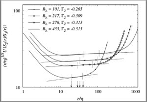
(7) $\begin{equation*}\left | \frac{S_n(r)}{S_3(r)}\right |\sim r^{\Gamma_n}, \qquad \mbox{where} \quad \Gamma_n= \zeta_n - \zeta_3. \end{equation*}$

Results were obtained only for the case $n=2$ and figures 9 and 10 from [1] are of interest, and are reproduced here. The first of these is the plot of the compensated ratio $(r/\eta)^{1/3}U|S_2(r)/S_3(r)|$ against $r/\eta$ , where $\eta$ is the dissipation length scale and $U$ is the rms velocity. This illustrates the way in which the exponents were obtained.

In the second figure, we show the variation of the exponent $\Gamma_2 + 1$ with Reynolds number, compared with the variation of the ESS exponent $\Sigma_2$ . It can be seen that the first of these tends towards the K41 value of $2/3$ , while the ESS value moves away from the K41 result as the Reynolds number increases.

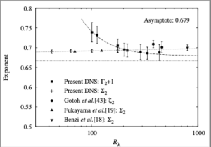Both methods rely on the assumption $\zeta_3 =1$ , hence $\Gamma_2+1 = \zeta_2$ , which is why we plot that quantity. We may note that figures 1 and 2 point clearly to the existence of finite Reynolds number corrections as the cause of the deviation from K41 values. Further details and discussion can be found in reference [1].

[1] W. D. McComb, S. R. Yoffe, M. F. Linkmann, and A. Berera. Spectral analysis of structure functions and their scaling exponents in forced isotropic turbulence. Phys. Rev. E, 90:053010, 2014.

Nov 4, 2021

The second-order structure function corrected for systematic error. / David McComb on the Physics of Turbulence by blogadmin is licensed under a Creative Commons Attribution CC BY 3.0

Leave a Reply Cancel reply

Report this page