

Viscous and forcing corrections to Kolmogorov’s ‘4/5’ law.
The Kolmogorov `4/5′ law for the third-order structure function  is widely regarded as the one exact result in turbulence theory. And so it should be: it has a straightforward derivation from the Karman-Howarth equation (KHE), which is an exact energy balance derived from the Navier-Stokes equation. Nevertheless, there is often some confusion around its discussion in the literature. In particular, for stationary isotropic turbulence, there can be confusion about the effects of viscosity (small scales) and forcing (large scales). These aspects have been clarified by McComb et al [1], who used spectral methods to obtain
  and
and  from a direct numerical simulation of the equations of motion.
If we follow the standard treatment (see [2], Section 4.6.2), we may write:
(1) 
In the past, this statement has been criticised because it omits the forcing which must be present in order to sustain a stationary turbulent field. However, it should be borne in mind that this is an entirely local equation; and, if the effect of the forcing is concentrated at the largest scales, then omission of these scales also omits the forcing. We can shed some light on this by reproducing Figure 7 from [1], thus:
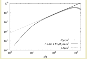
The results were taken at a Taylor-Reynolds number  , and show how the departure from the `4/5′ law at the small scales is due to the viscous effects. Clearly there is a range of values of
  where the `4/5′ law may be regarded as exact, in the ordinary sense appropriate to experimental work. This range of scales is, of course, the inertial range. Note that
  is the Kolmororov length scale.
Presumably the departure from the `4/5′ law at the large scales is due to forcing effects, and McComb et al [1] also shed light on this point. They did this by working in spectral space, where stirring forces have been studied since the late 1950s in the context of the statistical theories (e.g Kraichnan, Edwards, Novikov, Herring: see [3] for details) and are correspondingly well understood. They began with the Lin equation:
(2) 
where in principle the energy and transfer spectra depend on time, whereas the spectrum of the stirring forces  is taken as independent of time in order to ensure ultimate stationarity. Thus we will drop the time dependences hereafter as we will only consider the stationary case.
We can derive the KHE from this and the result is the usual KHE plus an input term  , defined by:
(3) 
where  is the three-dimensional Fourier transform of the work spectrum . By integrating the KHE (as Kolmogorov did in deriving the `4/5′ law) we obtain the form for the third-order structure function as:
(4) 
where where  is given in terms of the forcing spectrum by:
(5) ![\begin{equation*} X(r) = -12r\int_0^{\infty}\,dk W(k)\,\left[\frac{3\sin kr - 3kr \cos kr-(kr)^2 \sin kr}{(kr)^5}\right].\end{equation*}](https://blogs.ed.ac.uk/physics-of-turbulence/wp-content/ql-cache/quicklatex.com-f38f90f221a105551fdd4fc9f7c3217b_l3.png "Rendered by QuickLaTeX.com")
The result of including the effect of forcing is shown in Figure 8 of [1], which is reproduced here below.
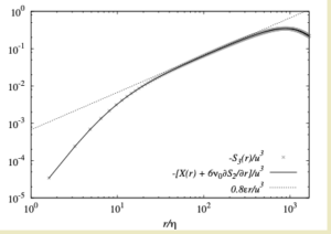
These results are taken from the same simulation as above, and now the contributions from viscous and forcing effects can be seen to account for the departure of from the `4/5′ law at all scales.
In [1] it is pointed out that is not a correction to K41, as used in other previous studies. Instead, it replaces the erroneous use of the dissipation rate of others’, and contains all the information of the energy input at all scales. In the limit of  forcing,
  , such that
  , giving K41 in the infinite Reynolds number limit. Note that
  is the rate of doing work by the stirring forces. Further details may be found in [1].
[1] W. D. McComb, S. R. Yoffe, M. F. Linkmann, and A. Berera. Spectral analysis of structure functions and their scaling exponents in forced isotropic turbulence. Phys. Rev. E, 90:053010, 2014.
[2] W. David McComb. Homogeneous, Isotropic Turbulence: Phenomenology, Renormalization and Statistical Closures. Oxford University Press, 2014.
[3] W. D. McComb. The Physics of Fluid Turbulence. Oxford University Press, 1990.

