

The infinite Reynolds number limit: Onsager versus Batchelor: 2
In the preceding post, we argued that the final statement by Onsager in his 1949 paper [1] is, in the absence of a proper limiting procedure, only a conjecture; and that the infinite Reynolds number limit, as introduced by Batchelor [2] and extended by Edwards [3], shows that it is incorrect. It is indeed possible to formulate the limiting case such that the detailed symmetry, which guarantees energy conservation by the nonlinear term, is preserved globally. At this point we should note that such extreme limits can only be taken in the context of continuum mechanics, but not for a real physical fluid, where the equation of motion is derived from statistical mechanics. There is also the question: how does the turbulence actually behave in the limit of infinite Reynolds numbers?
We may address these two points together by introducing the flux  of energy through the mode with wavenumber
  , thus:
(1) 
where  is the energy transfer spectrum, as it appears in the Lin equation, and we have assumed stationarity for sake of simplicity.
As is well known, the effect of increasing the Reynolds number is to increase the flux until it reaches a maximum value equal to the rate of dissipation  . We may write this as:
(2) 
Thereafter, as we increase the Reynolds number, the flux cannot increase any further, but the dissipation wavenumber keeps increasing, and the above relationship applies over an increasing range of wavenumbers. This is known as scale-invariance and in effect defines the inertial range. We now write the Edwards result for the infinite Reynolds number limit as:
![\[T(k) = \varepsilon_W \delta (k) -\varepsilon \delta (k-\infty) \equiv \varepsilon \delta (k) -\varepsilon \delta (k-\infty), \]](https://blogs.ed.ac.uk/physics-of-turbulence/wp-content/ql-cache/quicklatex.com-4f50eaedeb9b932f1b99e204e0f68381_l3.png "Rendered by QuickLaTeX.com")
where  is the rate of doing work by arbitrary stirring forces. Then, trivially, substituting this into equation (1) shows that it is mathematically equivalent to scale-invariance.
For many years, it has been widely accepted among theorists that the onset of scale-invariance is in effect the onset of infinite Reynolds number behaviour. Both numerical simulations and computations of statistical closures alike have shown the asymptotic behaviour
![\[\lim_{R\rightarrow \infty}\frac{\varepsilon_T}{\varepsilon} \rightarrow 1,\]](https://blogs.ed.ac.uk/physics-of-turbulence/wp-content/ql-cache/quicklatex.com-a06aac7fab3c2da156f0650ff0876e63_l3.png "Rendered by QuickLaTeX.com")
from below. Here we show the reciprocal of this behaviour (because we were studying the dissipation at the time) where we plot the ratio of dissipation to maximum flux against Taylor-Reynolds number.
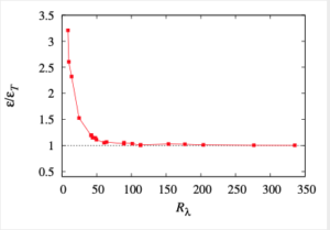
This figure is taken from the thesis [4] and will appear in a paper now in preparation [5]. Clearly the ratio of dissipation to maximum flux  approaches unity from above, as the Reynolds number increases. Evidently from about
  , scale-invariance is well established. In the next post, we shall discuss the nature of viscous dissipation and distinguish it from quasi-dissipation.
[1] L. Onsager. Statistical Hydrodynamics. Nuovo Cim. Suppl., 6:279, 1949.
[2] G. K. Batchelor. The theory of homogeneous turbulence. Cambridge University Press, Cambridge, 2nd edition, 1971.
[3] S. F. Edwards. Turbulence in hydrodynamics and plasma physics. In Proc. Int. Conf. on Plasma Physics, Trieste, page 595. IAEA, 1965.
[4] S. R. Yoffe. Investigation of the transfer and dissipation of energy in isotropic turbulence. PhD thesis, University of Edinburgh, 2012.
[5] W. D. McComb and S. R. Yoffe. The inifinite Reynolds number limit and the quasi-dissipative anomaly. (In preparation: 2020)

