Formulation of Renormalization Group (RG) for turbulence: 1

Formulation of Renormalization Group (RG) for turbulence: 1

In my posts of 30 April and 7 May, I discussed the relevance of field-theoretic methods (and particularly RG) to the Navier-Stokes equation (NSE). Here I want to deal with some specific points and in the process highlight the snags involved in going from microscopic quantum randomness to macroscopic deterministic chaos.

The application of the dynamic RG algorithm to randomly stirred fluid motion was pioneered by Forster et al (FNS) [1] and what is essentially their algorithm (albeit in our notation) may be stated as follows.

Filter the velocity field $u(k,t)$ into $u^-(k,t)$ on $0\leq k \leq k_1$ and $u^+(k,t)$ on $k_1\leq k \leq k_0$ . Note that we introduce $\nu_0$ as the notation for the kinematic viscosity, thus anticipating the subsequent normalization. The RG algorithm then consists of two steps.

1. Solve the NSE on $k_1 \leq k \leq k_0$ . Use that solution to find the mean effect of the high- $k$ modes and substitute it into the NSE on $0 \leq k \leq k_1$ . This results in an increment to the viscosity $\nu_0 \rightarrow \nu_1 = \nu_0 + \delta \nu_0$ .

2. Rescale the basic variables so that the NSE on $0 \leq k \leq k_1$ looks similar to the original NSE on $0 \leq k \leq k_0$ .

These steps are repeated for $k_2 < k_1$ , $k_3 < k-2$ , and so on; until a fixed point which defines the renormalized viscosity is reached. The general idea is illustrated schematically in the figure.

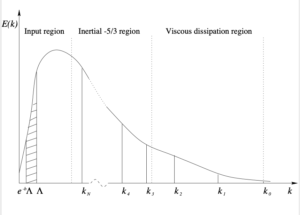
Sketch illustrating the choice of wavenumber bands for Gaussian perturbation theory at small wavenumbers and the choice of bands for recursive RG at large wavenumbers.

Two approaches are illustrated in the figure. First, we have the theory of FNS [1], in which a stirring force with Gaussian statistics is specified and an ultraviolet cut-off wavenumber $k_0 =\Lambda$ is chosen to be small enough to exclude the effects of the cascade. This means that this is not a theory of turbulence and the authors make that fact clear in their title. More recent workers in the field have not been so scrupulous. While FNS do obtain a fixed point, this is at $k=0$ , which is a trivial fixed point analogous to the high-temperature fixed point in critical phenomena.

The first version of my iterative-averaging theory was developed over the period 1982-86 and is summarised in [2]. Here the ultraviolet cutoff is chosen to be $k_0=k_max$ , such that the turbulence dissipation is approximately captured by the formulation, thus:

$\varepsilon \simeq \int^{k_{max}}_0 \, 2\nu_0 k^2 E(k) \,dk,$

where $E(k)$ is the energy spectrum [2]. The wavenumber bands are introduced through $k_1 = h k_0$ , where $h$ is the spatial rescaling factor, such that $0 \leq h \leq 1$ , and the bandwidth is given by $\eta = 1-h$ . In this approach the stirring forces are chosen to be peaked near the origin and are specified by their rate of doing work on the fluid. The RG iteration does not involve them in any way as it reaches a fixed point which corresponds to the top of the inertial range.

It is a cardinal principle of RG that the final result should not depend on the arbitrary parameters of the transformation. In the case of iterative averaging, the fixed point effective viscosity was found to be independent the choice of value $\nu_0$ , over quite a wide range. However, there was some dependence on the choice of $h$ and this was a signal that something was wrong.

The problem lay with the averaging. To simply filter and then average over the $u^+$ means that we are treating the $u^-$ and $u^+$ as independent variables. In the case of Gaussian variables, as considered by FNS, they are independent. But for the deterministic solutions of the macroscopic NSE, they cannot be independent variables. In fact, it is not even possible to formulate a rigorous conditional average.

This is easily seen (although it took many years to see it!). The $u^-$ and the $u^+$ each consists of a filter function and a Fourier transform operating on the identical $u(x,t)$ . It is only the latter which is averaged. So if we average one, we average the other.
In order to get round this difficulty, we have to formulate the conditional average as an approximation and exploit the underlying idea of deterministic chaos. We shall discuss this in the next post.

[1] D. Forster, D. R. Nelson, and M. J. Stephen. Large-distance and long-time properties of a randomly stirred fluid. Phys. Rev. A, 16(2):732-749, 1977.
[2] W. D. McComb. Application of Renormalization Group methods to the subgrid modelling problem. In U. Schumann and R. Friedrich, editors, Direct and Large Eddy Simulation of Turbulence, pages 67{81. Vieweg, 1986. 25.
[3] W. D. McComb. Theory of turbulence. Rep. Prog. Phys., 58:1117{1206, 1995.
[4] W. D. McComb. Asymptotic freedom, non-Gaussian perturbation theory, and the application of renormalization group theory to isotropic turbulence. Phys. Rev. E, 73:26303-26307, 2006.

Sep 24, 2020

Formulation of Renormalization Group (RG) for turbulence: 1 / David McComb on the Physics of Turbulence by blogadmin is licensed under a Creative Commons Attribution CC BY 3.0

Leave a Reply Cancel reply

Report this page