

Operational Large-Eddy Simulation.
When I was visiting TU Delft in 1997, I stayed with my wife and daughter in the Hague, where we rented an apartment from one of the professors at Delft. He and his wife occupied the penthouse above us. They had originally bought the second apartment so that their teenage daughters could combine a degree of freedom with parental oversight. By the time we came, their girls had long since left home and they were renting it out to visiting academics.
My landlord (I’ll call him Brian, because that was his name) used to give me a lift into the campus in the mornings and this could be a nerve-racking experience. His car had once belonged to Queen Juliana and was a gigantic Cadillac (I think) that was fitted with every conceivable luxury. But Brian was rather a small man and had to drive while peering through the steering wheel, so that when he swept out of the apartment block and turned into the narrow street beside a canal, there seemed to me to be a good chance that we would end up in the water.
However, one day he took me to see his experimental rigs. These were in a vast hangar and were heavily insulated, so that to me they just looked like large shapeless lumps wrapped in something like kitchen foil. I was unable to muster much enthusiasm and Brian told me that I `had no soul’! On a later occasion, he remarked tartly that he didn’t see the point of turbulence theory as he would just use the computer if he needed to take turbulence into account. That, I thought, would come as a surprise to those engineers whose field is turbulence modelling, but his remark stayed with me and I wondered whether one actually could use the computer in some operational way to model turbulence.
In Edinburgh, at that time, we were studying large-eddy simulation of the energy spectrum in the context of RG, and using DNS to test ideas. A typical approach was to run a fully resolved simulation (say with  mesh points), with maximum wavenumber
  , and compare this with a low-wavemumber part simulation, cut off at
  , having in this case
  . As energy spectra invariably showed an upturn near the maximum wavenumber (exaggerated on a log scale), it seemed likely that an unresolved simulation would show a marked upturn and that removing this could be made the basis of a feedback mechanism to produce the `correct spectrum’ in which the velocity field was reduced proportionally.
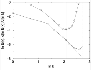
When back in Edinburgh, I discussed this with one of my students, who was working on DNS at the time. In [1] you can see how Alistair turned these vague ideas into an algorithm that worked. Referring to the figure below, this shows a spectrum for , where we introduce the wavenumber  to mark the point where the unresolved spectrum starts to turn up. That is the uncorrected spectrum and its derivative is used to identify the position of .
 and
and  respectively.
In the second figure, we show a comparison between the corrected and uncorrected spectra for , along with the spectrum for the resolved simulation with . It is clear that the compensated spectrum agrees well with the fully resolved one over their common range of wavenumbers.
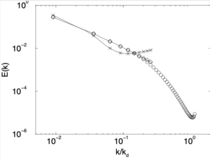
 simulation (circles), the unresolved
  simulation and the compensated simulation (diamonds).
For further details you should consult reference [1]. However, we can make a two specific points here.
First, the ratio  is plotted as a function of time in the paper. It was later pointed out to me that this is probably a good measure of eddy noise and that it would be interesting to know the form of its pdf. Unfortunately we did not think of measuring that at the time and anyone who is interested in subgrid modelling might find it helpful to rectify this omission. Another point in passing is that Fig. 2 in reference [1] shows a very rapid burst of activity at one stage and somehow this underlines just how little we really understand about the NSE as a dynamical system.
Secondly, when the subgrid drain due to the feedback loop is interpreted as a subgrid eddy viscosity, this agrees closely with the usual phenomenological form based on the truncated transfer spectrum and the corresponding energy spectrum. See Fig. 5 in reference [1].
Of course one would like to apply such a method to shear flows, but there the picture is complicated by the fact that lack of homogeneity means that energy can flow due to inertial transfer in space as well as in wavenumber. One could study this by separating the two effects, using centroid and relative coordinates. If spatial transfer were mainly due to large eddies, then a practical separation might be achieved.
[1] A. J. Young and W. D. McComb. Effective viscosity due to local turbulence interactions near the cutoff wavenumber in a constrained numerical simulation. J. Phys. A, 33:133-139, 2000.

