

Since the introduction of blockchain systems more than a decade ago, groups and individuals from both academia and industry have strived to refine the underlying protocols, improving their scalability, stability or decentralisation properties, to name a few. In this blog post, we will focus on the aspect of decentralisation and particularly on its dependence to system incentives. We examine the case of Cardano, a Proof-of-Stake blockchain whose design followed a first-principles approach, guided by research performed jointly with our Lab.
First, we will briefly explain how rewards are distributed in Cardano, and then we will examine several questions that arise in this reward scheme. For instance, how do we expect the stakeholders to engage with the protocol? Does the system converge to an equilibrium, i.e., a state where stakeholders have settled on their “strategies” and have no incentive to deviate from them? If yes, how many pools are there in this stable configuration of the system and how many independent stakeholders are behind these pools? In other words, how decentralised is the system at equilibrium?
To address these and more questions, we make use of a simulation engine that models the way stakeholders interact with the reward system under different conditions, and we carry out numerous experiments with it, examining the dynamics and the final outcomes of these interactions.
Rewards in Cardano
To motivate its stakeholders to engage actively with the protocol, Cardano employs a reward sharing scheme with capped rewards and incentivised pledging, introduced in an academic paper and backed by a game-theoretic analysis that establishes its ability to steer the system towards favourable states. According to this system of incentives, there is a pot of rewards that is distributed among block producers in fixed intervals and the share that each block producer receives depends on how much stake they possess as well as their performance during the consensus protocol execution.
Stakeholders often lack the resources to engage with the protocol on their own, hence they tend to collaborate with others, forming groups that are commonly known as pools in the context of blockchains. Acknowledging the economic sense and subsequent inevitability of resource pooling, the designers of Cardano incorporated an “on-chain” pooling mechanism that offers transparency, reduces friction and enables the system incentives to influence all pool members directly. A pool in Cardano consists of an operator, who is responsible for engaging with the protocol, and the delegators, who delegate their stake to the operator in exchange for a share of the pool’s rewards. The stake that the operator contributes to the pool is referred to as pledge, and together with the stake of the delegators they form the pool’s total stake.
Ignoring the variance introduced by the execution of the underlying consensus protocol, the volume of rewards that a well-performing pool receives depends on both its total size (stake) and its pledge. As illustrated in the chart below, if two pools have equal pledge, then the one with the higher total stake earns higher rewards (R2 > R1); if two pools have the same total size, then the one with the highest pledge has the advantage (R3 > R2); however, if the size of a pool exceeds the designated saturation point, then the rewards it receives are equal to those of a pool that has the same pledge and its size is exactly at the saturation point, i.e., it does not earn additional rewards for any stake beyond saturation (R5 = R4).
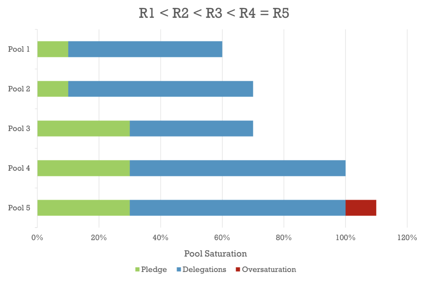 Note that if the rewards were not capped at the saturation threshold, then a pool would have incentive to increase its stake indefinitely, and, with resource holders naturally allocating their resources to the pools that get the highest rewards, the system could end up having very few “mega-pools” —or even a single one— with excessive leverage, and thus little to no achievement of decentralisation. A negative side-effect of capping is that it may create an incentive for some operators to run multiple pools. This is what the incentivised-pledging part of the mechanism aims to counterbalance: granting higher rewards to the pools with higher pledge is meant to encourage operators to keep their stake concentrated to one pool instead of splitting it across multiple pools (which could also manifest as a Sybil attack against the system). The specific cap that is used and the degree to which a pool’s pledge influences its rewards depend on protocol parameters, respectively k, which represents the target number of pools in the system, and a0 (we will discuss more about the impact of these parameters later in the post).
After the rewards are issued to a pool, the protocol is still responsible for their fair distribution to the pool members. From the total rewards of the pool, a fixed amount is first set aside for the operator, to offset the operational cost they have declared. From the remaining rewards, a fraction, equal to the profit margin the operator has set for the pool, is also allocated to the operator as compensation for the extra effort they put in. Finally, the rest of the rewards are distributed among all delegators, proportionally to the stake that each of them contributes. Note that the pool operator also receives delegation rewards, because of the stake they contribute to the pool (typically through pledging), which also counts towards its total stake.
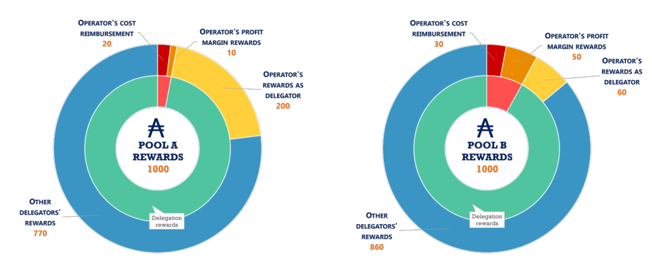
From the above description, we understand that a pool can be less or more attractive towards delegators depending on the deductions that are made to the pool’s rewards prior to distribution (in accordance with the pool’s operational cost and the profit margin selected by the operator). For example, the charts above show that Pool A and Pool B receive equal rewards from the protocol (1000 ADA), but different amounts end up being distributed to the delegators of each pool (970 in the case of Pool A and 920 in the case of Pool B); that is because Pool A has a lower operational cost (20 vs 30) and profit margin (1% vs 5%) than Pool B. Therefore, delegators need to pay attention to the properties of different pools before making their choice, in order to maximise their profits.
The Simulation
To confront the questions we posed earlier about the dynamics and the properties of the system, we developed a tool that simulates the behaviour of stakeholders in the Cardano reward scheme for various settings. To design this simulation engine, we first had to take a step back and observe the system in question, in the hope of building a model that captures its operation accurately.
In this context, we observe that the stake pool operation and delegation process of Cardano forms a socioeconomic complex adaptive system of heterogeneous stakeholders, who possess limited information each and interact directly and indirectly with other stakeholders and with their environment. In complex systems, the individual elements follow simple rules, yet the system itself behaves in a complex manner (i.e., its outcome is difficult to predict by looking at its elements in isolation). In our case, the behaviour of the stakeholders is restricted to operating stake pools or delegating stake to other pools, yet through a sequence of these simple actions, complex properties emerge for the system as a whole, such as its (in)stability or (de)centralisation.
In cases like this, it makes sense to use a “bottom-up” approach, i.e., model the individual elements of the system (micro-behaviour) and then observe the patterns that emerge (macro-behaviour), which is why we employ an agent-based model as the basis for the simulation. The goal of the individual agents is the generation of profit, while their behaviour (the way they choose what to do with their stake) follows rules and heuristics that help them reach this goal.
So how do agents choose their strategies in the simulation? First of all, by “strategy” we refer to what an agent does with their stake, so the possible strategies are to:
A) Operate a pool with a certain profit margin and use their stake as pledge
B) Delegate their stake to one or more pools
When considering operating a pool, an agent needs to decide on a value for its profit margin, which is the fraction of the pool’s profits that is set aside for the operator before any further distribution. At first thought, it may seem that the higher the margin, the higher the operator’s profits will be. However, as mentioned earlier, a pool with a high margin is typically less likely to attract delegations than a pool with a low margin, and pools need delegations to increase their stake and earn higher rewards; therefore, the pool operators need to find a balance between having a margin low enough to attract delegations and having a margin high enough to allow for increased profit. In the simulation, we capture this by having agents compare the potential profit of their pool with that of all other active pools and deciding on a margin that keeps their pool competitive in the eyes of prospective delegators.
When considering which pool to delegate their stake to, a stakeholder examines the different active pools in the system and estimates which pool will likely yield the highest rewards for them. From a delegator’s perspective, a pool is more attractive when it allows for a higher fraction of the rewards to be distributed among its members. Going back to the example we went through earlier where Pool A distributes 970 of the 1000 rewards to its members and Pool B 920 of 1000, it is evident that a potential delegator would choose Pool A over Pool B, as they would receive a fraction of a bigger share that way¹.
This share, represented by the cyan part of each inner doughnut chart, expresses the desirability of a pool is in the eyes of the delegators². Delegators want to be members of pools with high desirability, therefore, upon their turn, the agents in our simulation rank the existing pools based on the volume of the rewards that they expect to be distributed to delegators and choose the highest-ranking ones to delegate their stake to, prioritising the ones that are not fully saturated.
When the simulation starts, there are no pools in the system; at every step, the agents take turns (at random) and decide on a strategy for how to use their stake, based on the state of the system at that point and any information that has been made public by the other agents.A round is completed when all agents have had the chance to change their strategy, and this process goes on, until they have all settled to a specific strategy, or until a predetermined number of rounds is exceeded.
We run multiple experiments using the simulation, to understand how the stakeholders behave in different settings and how the system evolves as a whole. In many of these experiments, we use a Pareto distribution to sample the stake values that the agents start off with, which is a standard methodology for modelling wealth distributions. We set the total rewards available in the system to be equal to 1 and for the costs of the agents we use a uniform distribution in the range of [10-5, 10-4], which means that the average cost for operating one pool is 5 ⁄ 100,000 of the total rewards³.
¹ Note that in real life, there are more factors to consider that could influence a delegator’s decision. For example, if Pool B is a mission-driven pool, donating part of their profit to charity, then a delegator might be happy to accept lower rewards.
² Observe that in this example, Pool A is more desirable than Pool B even though the operator of Pool A receives overall more rewards. This is because the higher share that the operator receives through their delegation does not affect negatively the share of the other delegators (it only means that there is less space for delegations until saturation), therefore it is irrelevant for the delegators in this aspect.
³ These values were chosen as being somewhat in line with the real-world cost / reward ratios in Cardano but experiments were also conducted with different values.
System Evolution – Pool Splitting
Previous attempts at simulating staking behaviour in this context have revealed that over time the system stabilises to an equilibrium with k pools of equal size, regardless of the specific values used for the system’s parameters and under different assumptions about its initial state (see Section 7 of the relevant paper for details). However, these experiments assumed that each stakeholder could operate at most one pool, therefore it remained unclear whether the system would produce similar results in an environment where an agent has the capacity to operate multiple pools at any time –which, importantly, is the case in real life.
As discussed above, the reward mechanism of Cardano imposes an upper bound to the rewards that a pool can receive, thus disincentivising the formation of very large pools whose operators exert excessive power within the system. Be that as it may, there is still concern that individuals can circumvent this measure and gain disproportionate control over the system by operating multiple pools. This behaviour has become known as pool splitting, since operators usually start off with one pool, which they later split into two or more pools, if they deem it profitable. In theory, the pledging mechanism exists to deter pool-splitting behaviours in this setting, but how does it play out in practice?
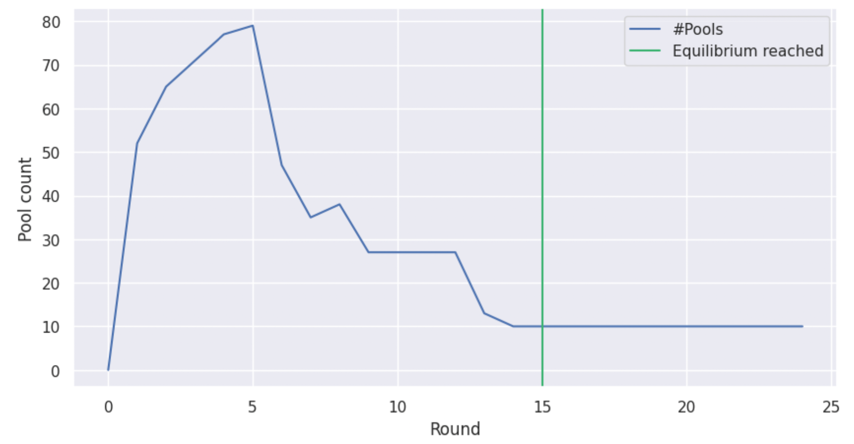
Hence, an important part of the work we are presenting here was to integrate multi-pool strategies in the simulation environment, to enable us to study the emergence and impact of pool-splitting behaviours. Having done that, we run the simulation and observe the results, starting with the following graph, which shows the number of active pools in the system for several rounds, until an equilibrium is reached. Note that for the experiments of this section, we used n = 1000 stakeholders in the system and a low k = 10 for the number of desirable pools –primarily for illustration purposes– but later sections cover bigger experiments as well.
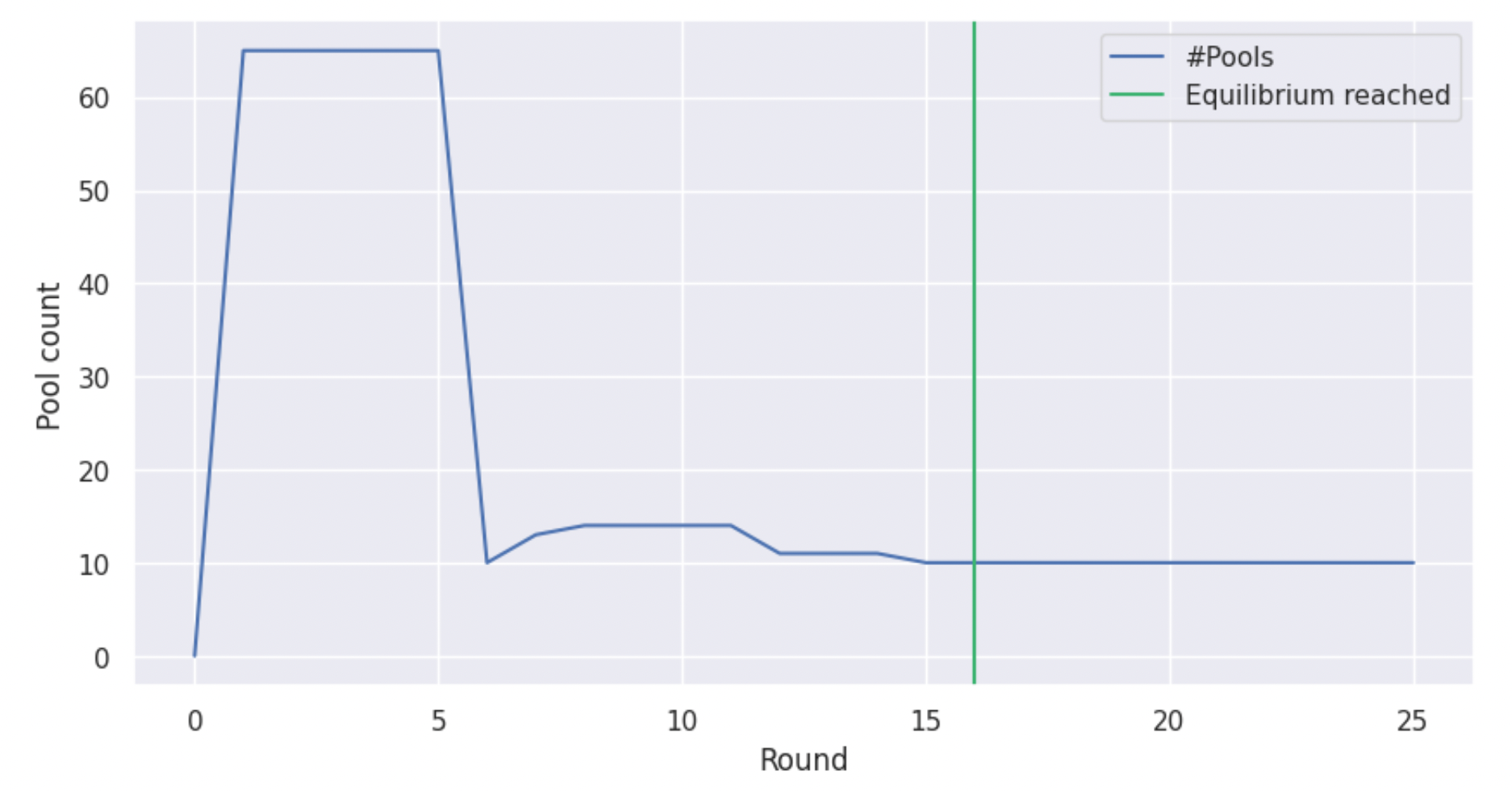
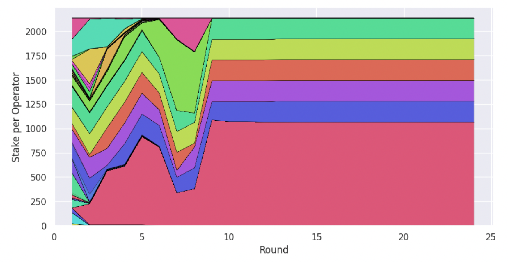
From the graph above, we see that the system indeed converges to k pools, in line with the previous experiments and despite pool splitting. Furthermore, we observe that there is a surge in the creation of pools during the first steps of the simulation, as agents “try their luck”, but in the end only few pools remain. The above graph doesn’t reveal two important things though. First, is the stake of the system evenly distributed among the pools or does a minority of the pools control the majority of the stake? Second, are these k pools independently owned or are there agents who managed to control a number of pools all the way to the equilibrium? To answer these questions, we construct another graph, which shows for every round how much stake is allocated to each stakeholder through pools that they own.
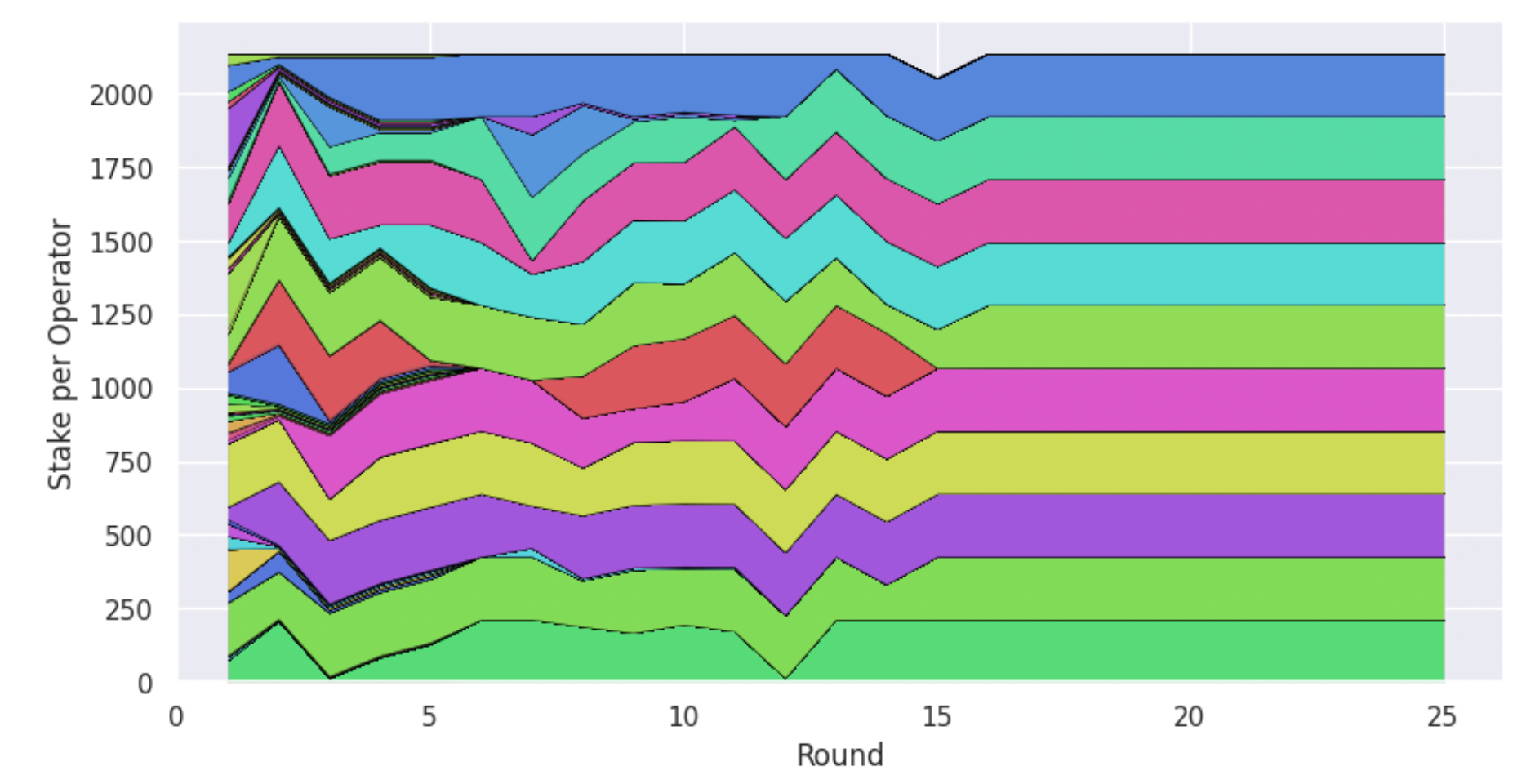
As we can see, all agents that end up as pool operators control equal stake through their pools. We also observe that there are 10 entities that control stake at the equilibrium, which we know from the previous graph is equal to the number of pools, therefore we can deduce that there is no pool splitting taking place there. These results are very encouraging, and they indicate that the system’s degree of decentralisation can be controlled through its parametrisation. However, this is but one example with specific values for the system’s parameters.
Earlier, we spoke about incentivised pledging in Cardano in the sense that the more stake a pool operator pledges to their pool, the more rewards the pool will receive. How much more though? This depends on the protocol parameter a0 (the higher the value of a0 the higher the influence of the pledge in determining the total rewards of the pool). In the previous example, we used a0 = 0.3, which is the value that the parameter currently holds in Cardano’s live system. It appears that for the conditions we have modelled above, this value is sufficient to deter pool splitting. What happens though when we use a much lower value for this parameter? In that case, decreasing the pledge of a pool may not lower its rewards sufficiently to provide a counterincentive against pool splitting. Using a0 = 0.003, we get the results that are illustrated in the graphs below.
The number pools stabilises yet again to 10, exemplifying the mechanism’s ability to induce convergence to k pools. However, tracking the allocation of stake per independent entity, we observe a very different story than last time. Now, there are agents who attempt to split their stake and operate multiple pools, throughout the course of the simulation. Not all of them are successful, but in the end a single operator is left in charge of half of the active pools (and half of the active stake), which is not a desirable outcome.
Measuring decentralisation: Nakamoto coefficient
We saw that the value of the a0 parameter of the reward mechanism can have a tremendous impact on the behaviour of the agents and the eventual pool structure of the system. This begs the question, what happens if we change the other parameter related to the rewards, the number of desired pools k? How can we find a combination of values for these parameters that encourages decentralisation? To gain insight on the conditions necessary to achieve a favourable outcome, we first need to find a concise way to represent a simulation execution based on its eventual degree of decentralisation, and then run numerous experiments with different combinations of parameters.
A popular metric that was proposed for quantifying the vague concept of decentralisation is the Nakamoto coefficient. The Nakamoto coefficient represents the minimum number of independent entities that collectively control more than 50% of the network’s resources (and could therefore launch a 51% attack against the system and subvert transactions if they colluded). In the context of Proof-of-Stake, this translates to controlling the majority of the active stake. In our toy examples from above with k = 10, the Nakamoto coefficient would be 6 in the case of the higher a0 and 2 in the case of the lower one.
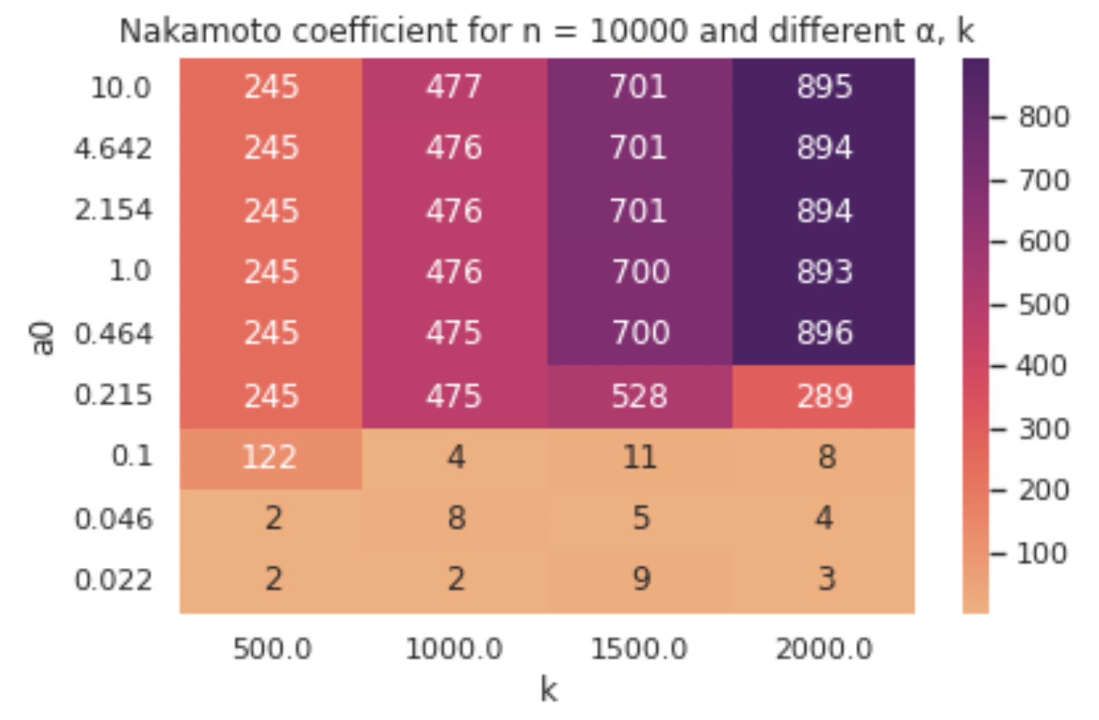
We run the simulation for a set of different parameter combinations in a suitable range, to determine when we get the most desirable results. In the heatmap below, each cell represents the Nakamoto coefficient of the final state of a simulation run with a certain k and a0.
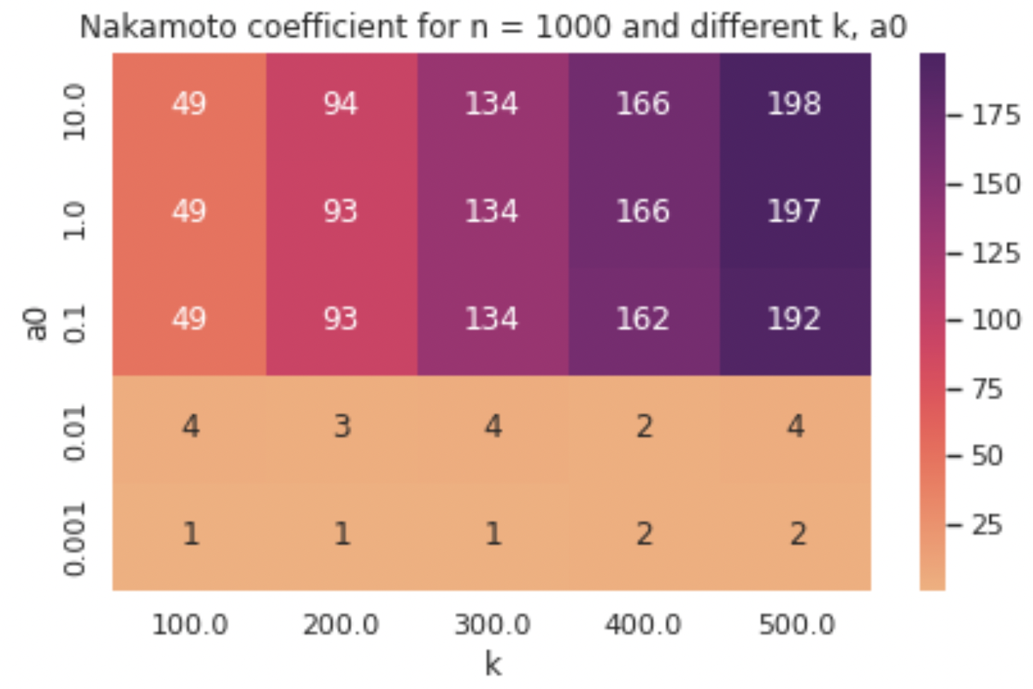
We observe that a very low a0 is not sufficient to deter pool splitting, resulting in an unacceptably low Nakamoto coefficient, with only a handful of independent operators (or even just one in some cases) controlling the majority of the stake through their many pools. From a point on (0.1 in the case of this experiment), a0 becomes effective and we see the Nakamoto coefficient jump to a good range of values. Any value above the threshold where the phase transition occurs is theoretically a good value for a0, however two things should be considered before making such a choice.
First, choosing a very high value for a0 is not desirable, as there are disadvantages that come with that which cannot be seen from our graphs. Even though a high a0 value would provide a robust defence against pool splitting and Sybil attacks, it would also impose a higher barrier to entry, as agents with limited stake would not be able to earn high rewards for their pools, while “rich” stakeholders would remain competitive, receiving much higher rewards for their high-pledged pools. This trade-off between Sybil resilience and egalitarianism is vital to keep in mind when selecting the parameter values of a real-world system. We also note that the increase in a0 past the threshold only yields a slight increase in the Nakamoto coefficient, if any, therefore there is no need to set a value for the parameter much higher than its threshold value (though it’s vital not to set it below the threshold value, which makes the optimal choice non-trivial).
Similarly for the k parameter, we observe that a higher value typically results in a higher Nakamoto coefficient in our experiments, but there are a couple of things we can remark for that as well. First, we observe that when a0 is low (0.001 and 0.01 in our experiments), then k only has a marginal impact, if any, as it can’t help with controlling pool-splitting behaviours. For an acceptable value of a0, such as 0.1 or larger, the increase of k does trigger a substantial increase in the Nakamoto coefficient, confirming that a change in k can aid in boosting the decentralisation of the system.
However, even though it’s tempting to think that “the higher the k value the better”, there are a few reasons why this may not always be the case. One caveat is that there is a natural limit on the number of stakeholders that can become pool operators, imposed by the combinations of stake and operational cost that they have to begin with. For some stakeholders with high costs, operating a pool may never be profitable, independent of the value of 𝑘. Once this limit is exceeded, the degree of decentralisation will plateau, or even drop, as the most profitable stakeholders expand their pools to fill the shoes of the ones who couldn’t make it. Note that in the real world, there are even more reasons besides the lack of profitability as to why a stakeholder would not become a pool operator, such as the lack of time or technical knowledge required to set up and maintain a stake pool.
Another remark one can make from looking at the heatmap above is that while higher values of a0 result in high values of the Nakamoto coefficient, these values do not reach the “ideal” Nakamoto coefficient we would expect to get if the system converged to k independently owned pools of equal stake. In this ideal scenario, the Nakamoto coefficient is equal to k/2 + 1, like it was for our first toy example with k = 10. In the bigger experiments though, we notice that the Nakamoto coefficient is always a bit lower than the ideal one –a divergence which only widens while k grows. For example, for k = 100 we get 47 instead of the ideal 51 and for k = 200 we get 88 instead of 101.
The root cause of this issue is the skewed distribution of wealth that the agents start with. Remember that we sampled values from a Pareto distribution to allocate stake to the agents at the beginning of the simulation. Though this assumption brings the simulation closer to the real-life system, it also introduces an inherent bias for the configuration of pools at equilibrium. For example, if there are stakeholders whose initial stake is close to or even exceeds the saturation point of a pool, it is rational for these agents to create multiple pools during the course of the simulation, even when the Sybil resilience parameter a0 is high. We cannot blame the mechanism in these cases, as there is only so much that can be done with such a biased input; in fact, the results from the heatmap above are very encouraging, given the skewed distribution of stake that we assume.
To validate the hypothesis that the divergence from the ideal Nakamoto coefficient is caused by the shape of the initial stake distribution, we run the simulation with a different distribution, making sure this time that all agents start off with the same volume of stake —thus eliminating the input bias. The results in terms of Nakamoto coefficient of the final configurations can be seen in the heatmap below.
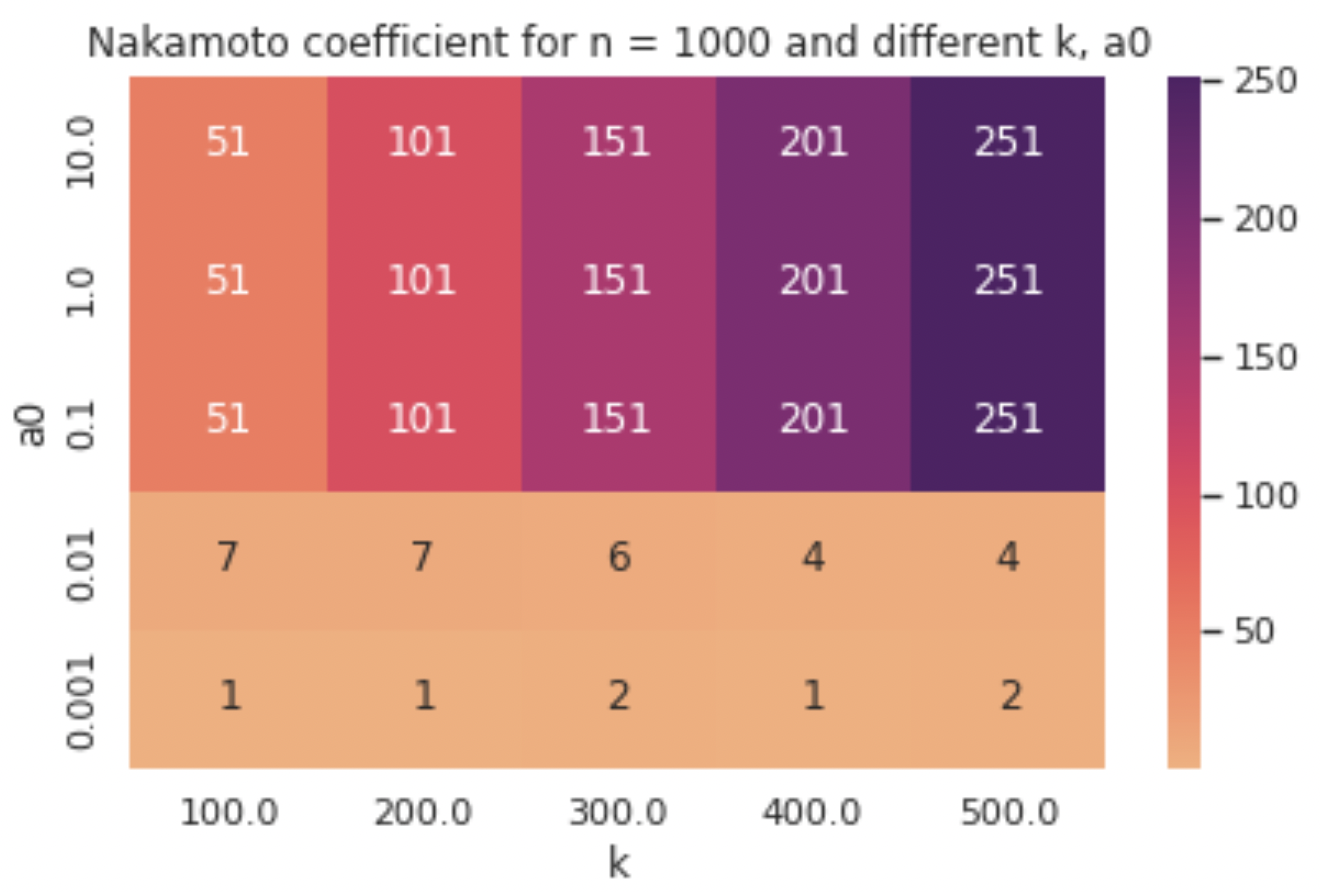
Once again, it is established that low values of a0 do not pose sufficient disincentives for pool splitting, allowing for a mere few operators to gain control of the majority of the system’s stake. However, this time we observe that for higher values of a0 we get the “ideal” Nakamoto coefficient, suggesting that the mechanism worked exactly as it was meant to and k pools of equal stake were formed in every one of these 15 simulation runs. This also serves as a reminder that all results that we discuss here are dependent on the stakeholder distribution that we feed into the simulation and the Pareto distribution that we have used up to now may not capture the real-world deployment distribution where more complex patterns can manifest in the context of staking (e.g., when many thousands of users participate and even cluster together off-chain or borrow stake in order to launch pools). Yet, the experiments above still provide a good indication of the effectiveness of the reward scheme in question (note that the numbers presented in the heatmaps above are the averages across a number of simulation runs with these parameter settings for various random seeds).
To capture the complexity of the real-world deployment, we perform two additional experiments.
First, we increase the number of stakeholders from 1,000 to 10,000 and show how the Nakamoto coefficient responds to a wider range of a0 values and to higher values of k. A notable result here is that in some cases (ostensibly when the value of a0 is on the border of being effective) we can observe the “upper bound” for the k parameter that we discussed earlier, after which the Nakamoto coefficient takes a dive (in the table below observe the row corresponding to a0 = 0.215).
Second, we run an experiment with a specially crafted initial stakeholder distribution that captures essential features of the currently live Cardano stakeholder distribution. Specifically, we design a synthetic stake distribution aimed to emulate the current Cardano stakeholder distribution, using a combination of real data points (taken from ADApools and PoolTool) and synthetic points that we draw from a Pareto distribution. Notably, we mark close to 1/4 of the total stake in the system as inactive, meaning that it is held by agents that abstain from staking, and we provide explicit stake values for a number of stakeholders that were identified by ADApools as cryptocurrency exchanges (e.g. Binance), named entities (e.g., IOG or Emurgo) and custody services.
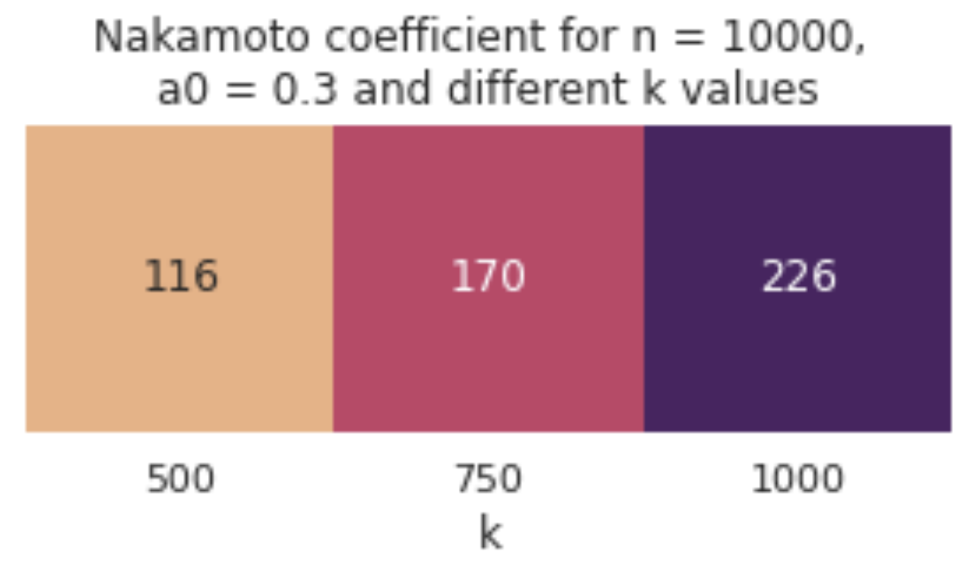
We use n = 10,000 agents and a0 = 0.3 (which is the value currently used in Cardano) and we compare some options for k, starting with the value currently used in the system (k = 500) and going up to the one that has been proposed for update (k = 1000). As expected, the values of the Nakamoto coefficient diverge more from the ideal ones, but the increase in k still helps to achieve a higher degree of decentralisation, as can be seen in the table below. Note that the final number of pools was also lower than k in these observations, which can be attributed to the decrease in the system’s active stake.
Key takeaways
In this blog post, we presented experimental results about the dynamics and equilibrium properties of staking in the Cardano rewards system. In particular, we tracked a behaviour that is of special interest to the Cardano community, pool splitting, and we demonstrated under which conditions it is expected to emerge, and how it can be controlled by the parameterisation of the scheme.
The results we obtained are in line with the theoretical claims made in the paper that introduced Cardano’s Reward Sharing Scheme, and can be summarised as follows:
- In the case of full participation, the simulation reaches an equilibrium with ~k pools (which is the desirable number of pools according to the reward scheme) even when agents are allowed to operate more than one pool each. When participation is smaller, this affects the number of pools at equilibrium in equal proportion.
- Whether stakeholders succeed in pool-splitting depends strongly on the value of the reward scheme’s a0 parameter. Adjusting suitably a0 and k can drive the system towards a more decentralised state, as measured by its Nakamoto coefficient.
- The degree to which it is possible to approximate the maximum possible value for the Nakamoto coefficient depends also on the initial distribution of stake across the stakeholders. This distribution, in the context of our simulations, is assumed to include any possible exchange of stake and organisation between them in anticipation of the staking process.
It is important to highlight that our results are based on simulations using an agent-based model that assumes strict utility maximizing behaviour on behalf of all participants. Real world staking behaviour involves many other factors (such as inability to make an optimal staking choice or choosing a pool based on the operator’s status in the community or the pool’s mission) that we do not model.
As a final point, we are working towards making the simulation engine publicly available; the code and its internal workings is something that will be covered in a future blog post.
by Christina Ovezik & Aggelos Kiayias
Posted 19 April, 2022


I would be curious to know what the value of Nakamoto coefficient was for values of k above 1000. For example all the way up to a point where the Nakamoto coefficient decreases. The “upper bound” that you mentioned.
Does this occur just above k=1000 or is it far ahead (k=5000?) The starting conditions are very different from the previous simulations.
The distribution of rewards is essentially using the treasury to pay pool operators to run the decentralised network. If maximum decentralisation is a desireable goal, then shouldnt the system strive to increase this to a maximum.
Hi Nick, thanks for your question. We have observed from our experiments that the optimal value of k is different depending on the initial distribution and the value of a0 that we use. For example, in our second-to-last experiment with the 10,000 agents and the Pareto distribution it seems that for a0 around 0.2 the optimal value for k is in the area of 1500, but this value increases with a0 and goes beyond the highest k value that we have modelled (2000).
I suppose your question is mainly about the last experiment with the synthetic stake distribution, for which we presented a more limited set of experiments. Unfortunately, I can’t give you a specific answer yet as to whether the “upper bound” of k comes soon after 1000 or not, but we are currently in the process of running more experiments with this distribution, so hopefully we’ll have more results to share soon. More importantly, we will be releasing the code of the simulation engine to the public, so that anyone who is interested can run their own experiments and share the results and their thoughts about them with the community 🙂
Thank so much for responding,
I’ll be interested in the results of those additional simulations with the synthetic stake distribution. It seems to me that you got a0 pretty much right already but that k could definitely be increased, probably to 2000 and beyond, without endangering decentralisation.
My judgement is that this would enable more pools to be viable and to offer increased decentralisation of the network. At no additional cost in funds used for incentivising operators to run pools.