Coding Confession of a Research Software Engineer

We all make mistakes. But they are quite often invisible. Especially when we are programming. Once we know that we have made a mistake we tend to fix it and move on to the next problem. Mistakes are a learning opportunity. Sharing them thus helps others. The Software Sustainability Institute is running a campaign to collect coding confessions.

Here is mine.

Computing the Gradient

A while ago I worked for a company as a research geophysicist developing software (that was well before the term research software engineer was coined). This is the story of me trying to compute the gradient on a non-regular grid.

Background

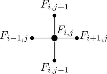
First of all some background. Let’s start with a regular mesh and calculate the gradient using finite differences.

Nodes in a regular mesh used for finite differences.

The forward difference is

$\frac{dF_f}{dx}\approx\frac{F_{i+1,j}-F_{i,j}}{\Delta x}$

and the backward difference is

$\frac{dF_b}{dx}\approx\frac{F_{i,j}-F_{i-1,j}}{\Delta x}$

Let’s take the mean of the forward and backward difference

$\frac{dF}{dx}\approx\frac12\left(\frac{dF_f}{dx}+\frac{dF_b}{dx}\right)=\frac{F_{i+1,j}-F_{i-1,j}}{2\Delta x}$

which is essentially the central difference. We can get a similar expression for the derivative with respect to y. We are going to use the same idea on an irregular mesh.

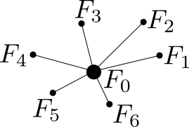
Finite differences on an irregular mesh

The neighbouring nodes are no longer connected along the x and y direction. We can still formulate forward differences, however, they are along the line connecting the two nodes:

$\frac{dF_0_i}{dr_i}\approx\frac{F_i-F_0}{|r_i|}$

However, we can express the derivative with respect to r as the sum of the derivatives with respect to x and y, ie

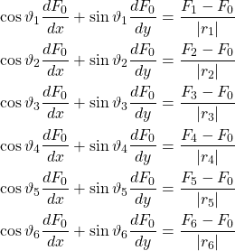
$\frac{dF_0_i}{dr_i} = \cos\vartheta_i\frac{dF_0}{dx} + \sin\vartheta_i\frac{dF_0}{dy}$

So, we now end up with a system of linear equations with two unknowns – the gradient we are interested in:

$\begin{align*} \cos\vartheta_1\frac{dF_0}{dx} + \sin\vartheta_1\frac{dF_0}{dy} &= \frac{F_1-F_0}{|r_1|}\\ \cos\vartheta_2\frac{dF_0}{dx} + \sin\vartheta_2\frac{dF_0}{dy} &= \frac{F_2-F_0}{|r_2|}\\ \cos\vartheta_3\frac{dF_0}{dx} + \sin\vartheta_3\frac{dF_0}{dy} &= \frac{F_3-F_0}{|r_3|}\\ \cos\vartheta_4\frac{dF_0}{dx} + \sin\vartheta_4\frac{dF_0}{dy} &= \frac{F_4-F_0}{|r_4|}\\ \cos\vartheta_5\frac{dF_0}{dx} + \sin\vartheta_5\frac{dF_0}{dy} &= \frac{F_5-F_0}{|r_5|}\\ \cos\vartheta_6\frac{dF_0}{dx} + \sin\vartheta_6\frac{dF_0}{dy} &= \frac{F_6-F_0}{|r_6|}\\ \end{align*}$

Excellent, this is an overdetermined system of equations which we can solve to find the gradient.

Attempt 1: use LAPACK

Solving an overdetermined system of equations is a standard problem. We can use the dgels routine from LAPACK to solve this problem. At the time we were already using the AMD Core Maths Library which comes with LAPACK. So, the problem was solved with a single function call. It turns out that that was a bad plan. Running the new routine millions of times took forever. The routine is optimised for large problems and allocates and deallocates memory for its work space. The problem at hand is tiny and the overhead of memory management totally overwhelmed any computations.

Attempt 2: Fortran to the rescue

This whole project was suitably old-school that we were using Fortran. The system of equations above can be rewritten as

$Ax=b$

where the coefficient matrix A contains all the cosine and sine terms and the vector b the finite differences. With some linear algebra we get

$\begin{align*} A^TAx&=A^Tb\\ x&=\left(A^TA\right)^{-1}A^Tb\\ &=B^{-1}A^Tb \end{align*}$

We can calculate the square matrix B using Fortran
B=matmul(transpose(A),A)
B is a 2×2 matrix which is easily inverted

$B^-1=\frac1{b_{11}b_{22}-b_{12}b_{21}}\left(\begin{matrix}b_{22} & -b_{12}\\-b_{21} & b_{11} \end{matrix}\right)$

A few more applications of the matmul function solved the problem. This was quite an improvement in runtime over the LAPACK method tried first. However, it was still too slow.

Attempt 3: pen and pencil

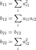
In the end I computed the elements of the 2×2 matrix B by hand rather than calling matmul:

$\begin{align*} b_{11} &= \sum_ia_{i1}^2\\ b_{12} &= \sum_ia_{i1}a_{i2}\\ b_{21} &= b_{12} \\ b_{22} &= \sum_ia_{i2}^2\\ \end{align*}$

using the sum function. The remaining matrix products were also computed in a similar manner using the sum function.

Lessons Learned

Although strictly speaking I didn’t make a mistake but I did produce unuseable code. The main lesson I learned was that I should know my tools. In the ideal world of mathematics it doesn’t matter so much how you arrive at a solution. In the world of scientific computing there can be make-or-break differences. Libraries are often optimised for particular use cases. In this case I was seduced by the label high performance, optimised LAPACK. Sadly, ACML is optimised for huge problems rather than my tiny problem. In the end the problem was solved using pen and paper and calls to simple functions.