Derivatives and Gaussian Processes

The general idea of machine learning is you take a set of data, train a model on it, and use this model to annotate new data. This could be to classify whether an image is of a cat or a dog, or to estimate the effect of changing a parameter in an experiment. In an abstracted version, you want to estimate the function values $y$ at new locations $x$ , given knowledge of what the function has done at other locations $z$ . But what if you also know what the derivative of the function is at $z$ ?

When working with physical systems we often know something about the derivatives: running watches come with accelerometers, and their readings can be combined with GPS data to improve the accuracy of location estimates. Combining several sources of data in this way is particularly helpful when there are few data points, and one method which allows you to include samples of the derivatives is Gaussian processes. Their additional advantage is that they provide uncertainty estimates. A standard neural network will tell you what its best guess is; a Gaussian process will give you an estimated mean and standard deviation. Due to their computational complexity they are best suited to small data sets – the ones which have most to gain from adding derivative information.

Last year, I found myself needing to work with derivative samples when using Gaussian Processes. I found references to the theory in several places, and this helpful discussion on Stackexchange, but I missed a step-by-step introduction. This blog post is meant to be what I wish I had found. I hope it might also be useful to someone else.

What are Gaussian Processes?

Gaussian Processes are a machine learning method used for regression, i.e. to determine the value at a new location given a set of known values. It works by assuming that all of the values come from a joint Gaussian distribution. Using this assumption, a specification of the expected mean and an assumption on the covariance between points, we can estimate values for a new set of points. The figure below gives two examples of this – one slowly-varying and one faster. The orange line shows the true function which the blue dots have been sampled from. The blue line shows the mean of the Gaussian Process prediction, and the shaded area shows points within one standard deviation of that mean.

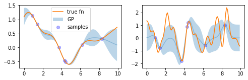
Two examples of Gaussian processes.

More technically, the blue areas and lines in the figure above have been calculated using equations 1. The first line states that the true function is assumed to come from a multivariate Gaussian distribution with mean $\bar{\boldsymbol{f}_*}$ and covariance matrix $\mathrm{cov}(\boldsymbol{f}_*)$ . The next two lines give expressions for calculating these. $X_\mathrm{n}$ is the matrix of feature vectors for the sampled points, and $X_*$ the same for the new points. $\mathrm{K}_{\mathrm{n}\mathrm{n}}$ , $\mathrm{K}_{**}$ and $\mathrm{K}_{*\mathrm{n}}$ are covariance matrices, calculated using a chosen covariance function $k(\cdot)$ ^[1]. $\mathrm{K}_{\mathrm{n}\mathrm{n}}$ is the covariance of the sampled points, $\mathrm{K}_{**}$ the covariance of the new points and $\mathrm{K}_{*\mathrm{n}}$ the covariance between these groups of points. $\sigma_\mathrm{n}$ is the standard deviation of the sampling noise, $\boldsymbol{\mathcal{I}}$ the identity matrix and $\boldsymbol{y}_{\mathrm{n}}$ the sampled values. For a thorough introduction to Gaussian Processes, see [1].

(1) $\begin{align*} \boldsymbol{f}_* | X_\mathrm{n}, \boldsymbol{y}_{\mathrm{n}}, X_* &\sim \mathcal{N} \left( \bar{\boldsymbol{f}_*}, \mathrm{cov}(\boldsymbol{f}_*) \right) \\ \bar{\boldsymbol{f}_*} &= \mathrm{K}_{*\mathrm{n}} \left( \mathrm{K}_{\mathrm{n}\mathrm{n}} + \sigma_\mathrm{n}^2 \boldsymbol{\mathcal{I}} \right)^{-1} \boldsymbol{y}_{\mathrm{n}} \label{eq-gaussian-predictions-b} \\ \mathrm{cov} (\boldsymbol{f}_*) &= \mathrm{K}_{**} - \mathrm{K}_{*\mathrm{n}} \left( \mathrm{K}_{\mathrm{n}\mathrm{n}} + \sigma_\mathrm{n}^2 \boldsymbol{\mathcal{I}} \right)^{-1} \mathrm{K}_{\mathrm{n}*} \label{eq-gaussian-predictions-c} \end{align*}$

An example

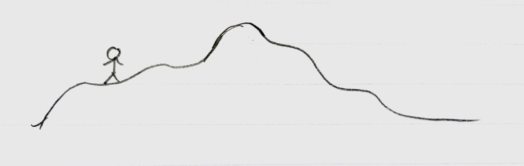
As an example, let’s consider the case of Harvey who is spending a day hiking. He doesn’t carry technology with him while hiking, but likes to estimate his altitude profile to put in his journal. To do so, he stops a couple of times during his trip and uses his map and his surroundings to estimate his altitude at that point. The rest of the time he is too busy avoiding falling off cliffs and enjoying the landscape to pay attention to his altitude.

Hiker Harvey preparing for his trip.

In a Gaussian Process context we can consider this a regression problem where we are trying to estimate the altitude throughout the day based on point estimates or samples. Let’s assume we have samples of the altitude at the start and end of the day, and also after two and four hours of walking, as shown in the plot below. Let’s order these points chronologically and call them $a$ , $b$ , $c$ and $d$ .

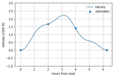
Plot of hiker Harvey’s altitude throughout the day, with samples indicated.

To model this with a Gaussian Process we need to specify a mean function and a covariance function. To keep this simple we will set the former to zero and use the version of the squared exponential kernel in equation 2 for the latter.

(2) $\begin{equation*} k(x_i, x_j) = \exp \left(-\frac{1}{2}(x_i-x_j)^2 \right) \end{equation*}$

Then, we need to compute the covariance matrices. This is done using the the covariance function, e.g. $\textcolor{blue}{\boldsymbol{\mathrm{cov}(a,b) }} = k(x_a, x_b)=\exp \left(-\frac{1}{2}(2)^2 \right)\approx\textcolor{blue}{\boldsymbol{0.14}}$ .

$\begin{equation*} \mathrm{K}_{\mathrm{nn}} = \begin{bmatrix} \mathrm{cov}(a,a) & \textcolor{blue}{\boldsymbol{\mathrm{cov}(a,b) }} & \mathrm{cov}(a,c) & \mathrm{cov}(a,d) \\ \mathrm{cov}(b,a) & \mathrm{cov}(b,b) & \mathrm{cov}(b,c) & \mathrm{cov}(b,d) \\ \mathrm{cov}(c,a) & \mathrm{cov}(c,b) & \mathrm{cov}(c,c) & \mathrm{cov}(c,d) \\ \mathrm{cov}(d,a) & \mathrm{cov}(d,b) & \mathrm{cov}(d,c) & \mathrm{cov}(d,d) \end{bmatrix} = \begin{bmatrix} 1.0 & \textcolor{blue}{\boldsymbol{0.14}} & 0.0 & 0.0 \\ 0.14 & 1.0 & 0.14 & 0.0 \\ 0.0 & 0.14 & 1.0 & 0.07 \\ 0.0 & 0.0 & 0.07 & 1.0 \end{bmatrix} \end{equation*}$

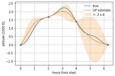
The covariance function is similarly evaluated to obtain $\mathrm{K}_{**}$ and $\mathrm{K}_{*\mathrm{n}}$ . Plugging the numbers into equations 1 we obtain the estimate in the below figure.

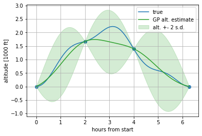
Harvey’s altitude throughout the day together with the estimate based on the four indicated samples.

Now add derivatives

The above examples only use samples of the function. However, it is also possible to incorporate knowledge through samples of the derivatives^[2]. Gaussian Processes work through specifications of the covariance between all points of interest. In particular, we need to know the covariance between all of our sample feature vectors, as well as between these and the location we’re interested in. If we want to include samples of the underlying process’ derivatives, we need a way of specifying the covariance between these derivative samples and the function samples. These covariances are the ones specified in equations 3 [1, p 191]. The first gives the covariance between two such samples of the derivative, and the second the covariance between a sample of the function and a sample of the derivative.

(3) $\begin{align*} \mathrm{cov} \left( \frac{\partial f_i}{\partial x_{di}}, \frac{\partial f_j}{\partial x_{ej}}\right) &= \frac{\partial^2 k(x_i, x_j)}{\partial x_{di} \partial x_{ej}} \\ \mathrm{cov} \left( f_i, \frac{\partial f_j}{\partial x_{dj}}\right) &= \frac{\partial k(x_i, x_j)}{\partial x_{dj}} \label{eq-der-two} \end{align*}$

$f_i$ and $f_j$ are two sample values and $x_i$ and $x_j$ are the corresponding feature vectors. $k(\cdot)$ is the specified covariance function. $x_{di}$ and $x_{ej}$ denote the value of the $d$ -th and $e$ -th dimensions of the feature vectors.

Continuing our example

So how does this work in practice? To illustrate, let’s imagine that Harvey not only estimated his altitude during his stops, but at the first one also estimated his vertical speed and acceleration. Accompanying code is available at https://github.com/sighellan/GP_derivatives_example.

Hiker Harvey on his way to the summit.

Our feature is the time $t$ ^[3], and the function we’re estimating is hiker Harvey’s altitude. Then the derivative is his vertical speed and the second derivative his vertical acceleration. We continue to use the squared exponential kernel as earlier, see equation 2.

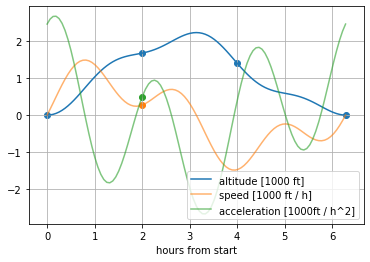
The altitude, vertical speed and vertical acceleration of hiker Harvey in our example, with samples indicated.

Since we are only using one feature dimension, we can drop some of the notation from equations 3, as given in equations 4.

(4) $\begin{align*} \mathrm{cov} \left( \frac{\partial f_i}{\partial x_{i}}, \frac{\partial f_j}{\partial x_{j}}\right) &= \frac{\partial^2 k(x_i, x_j)}{\partial x_{i} \partial x_{j}} \\ \mathrm{cov} \left( f_i, \frac{\partial f_j}{\partial x_{j}}\right) &= \frac{\partial k(x_i, x_j)}{\partial x_{j}} \label{eq-der-two-simp} \end{align*}$

To show how to use these samples, let’s continue to denote the altitude samples $a$ , $b$ , $c$ , $d$ , in chronological order. In addition, we’ll denote the speed sample $e$ and the acceleration sample $f$ . Then, what we need to do in order to calculate the covariance matrix $\mathrm{K}_{\mathrm{nn}}$ is written out explicitly in the matrix below.

$\begin{equation*} \mathrm{K}_{\mathrm{nn}} = \begin{bmatrix} \mathrm{cov}(a,a) & \mathrm{cov}(a,b) & \mathrm{cov}(a,c) & \mathrm{cov}(a,d) & \mathrm{cov}(a,e) & \mathrm{cov}(a,f) \\ \mathrm{cov}(b,a) & \mathrm{cov}(b,b) & \mathrm{cov}(b,c) & \mathrm{cov}(b,d) & \mathrm{cov}(b,e) & \mathrm{cov}(b,f) \\ \mathrm{cov}(c,a) & \mathrm{cov}(c,b) & \mathrm{cov}(c,c) & \mathrm{cov}(c,d) & \mathrm{cov}(c,e) & \mathrm{cov}(c,f) \\ \mathrm{cov}(d,a) & \mathrm{cov}(d,b) & \mathrm{cov}(d,c) & \mathrm{cov}(d,d) & \mathrm{cov}(d,e) & \mathrm{cov}(d,f) \\ \mathrm{cov}(e,a) & \mathrm{cov}(e,b) & \mathrm{cov}(e,c) & \mathrm{cov}(e,d) & \mathrm{cov}(e,e) & \mathrm{cov}(e,f) \\ \mathrm{cov}(f,a) & \mathrm{cov}(f,b) & \mathrm{cov}(f,c) & \mathrm{cov}(f,d) & \mathrm{cov}(f,e) & \mathrm{cov}(f,f) \end{bmatrix} \end{equation*}$

We see that some of these, namely the ones that only involve pairs of $a$ , $b$ , $c$ , $d$ , are calculated directly using the covariance function, and that we’ve already used them in our previous version of the problem. Below, I’ve filled in the covariance matrix with these values.

$\begin{equation*} \mathrm{K}_{\mathrm{nn}} = \begin{bmatrix} 1.0 & 0.14 & 0.0 & 0.0 & \textcolor{blue}{\boldsymbol{\mathrm{cov}(a,e)}} & \mathrm{cov}(a,f) \\ 0.14 & 1.0 & 0.14 & 0.0 & \mathrm{cov}(b,e) & \mathrm{cov}(b,f) \\ 0.0 & 0.14 & 1.0 & 0.07 & \mathrm{cov}(c,e) & \mathrm{cov}(c,f) \\ 0.0 & 0.0 & 0.07 & 1.0 & \mathrm{cov}(d,e) & \mathrm{cov}(d,f) \\ \mathrm{cov}(e,a) & \mathrm{cov}(e,b) & \mathrm{cov}(e,c) & \mathrm{cov}(e,d) & \mathrm{cov}(e,e) & \mathrm{cov}(e,f) \\ \mathrm{cov}(f,a) & \mathrm{cov}(f,b) & \mathrm{cov}(f,c) & \mathrm{cov}(f,d) & \mathrm{cov}(f,e) & \mathrm{cov}(f,f) \end{bmatrix} \end{equation*}$

Next, the covariances between $a$ , $b$ , $c$ , $d$ and $e$ can be filled in, e.g. $\textcolor{blue}{\boldsymbol{\mathrm{cov}(a,e)}} = \frac{\partial k(x_a, x_e)}{\partial x_{e}} = (x_a - x_e)k(x_a, x_e)=-2\exp \left(-\frac{1}{2}(2)^2 \right)\approx \textcolor{blue}{\boldsymbol{-0.27}}$ . Note that the jump between the second and third expression is only valid for our choice of covariance function. Filling in these yields

$\begin{equation*} \mathrm{K}_{\mathrm{nn}} = \begin{bmatrix} 1.0 & 0.14 & 0.0 & 0.0 & \textcolor{blue}{\boldsymbol{-0.27}} & \mathrm{cov}(a,f) \\ 0.14 & 1.0 & 0.14 & 0.0 & 0.0 & \mathrm{cov}(b,f) \\ 0.0 & 0.14 & 1.0 & 0.07 & 0.27 & \mathrm{cov}(c,f) \\ 0.0 & 0.0 & 0.07 & 1.0 & 0.0 & \mathrm{cov}(d,f) \\ -0.27 & -0.0 & 0.27 & 0.0 & \mathrm{cov}(e,e) & \mathrm{cov}(e,f) \\ \mathrm{cov}(f,a) & \mathrm{cov}(f,b) & \mathrm{cov}(f,c) & \mathrm{cov}(f,d) & \mathrm{cov}(f,e) & \mathrm{cov}(f,f) \end{bmatrix} \end{equation*}$

The above values could also be found in the Jacobian of the covariance function, and the covariances between $a$ , $b$ , $c$ , $d$ and $f$ as well as $\mathrm{cov}(e,e)$ can be found in the Hessian. The expressions are $\displaystyle \mathrm{cov}(a,f) = \frac{\partial^2 k(x_a, x_f)}{\partial^2 x_{f}}$ and $\displaystyle \mathrm{cov}(e,e) = \frac{\partial^2 k(x_i, x_j)}{\partial x_{i} \partial x_{j}}|_{i=e,j=e}$ . Using this, the matrix is now at

$\begin{equation*} \mathrm{K}_{\mathrm{nn}} = \begin{bmatrix} 1.0 & 0.14 & 0.0 & 0.0 & -0.27 & 0.41 \\ 0.14 & 1.0 & 0.14 & 0.0 & 0.0 & -1.0 \\ 0.0 & 0.14 & 1.0 & 0.07 & 0.27 & 0.41 \\ 0.0 & 0.0 & 0.07 & 1.0 & 0.0 & 0.0 \\ -0.27 & -0.0 & 0.27 & 0.0 & 1.0 & \mathrm{cov}(e,f) \\ 0.41 & -1.0 & 0.41 & 0.0 & \mathrm{cov}(f,e) & \mathrm{cov}(f,f) \end{bmatrix} \end{equation*}$

The final three covariances needed are $\displaystyle \mathrm{cov}(f,f) = \frac{\partial^4 k(x_i, x_j)}{\partial^2 x_{i} \partial^2 x_{j}}|_{i=f,j=f}$ , $\displaystyle \mathrm{cov}(e,f) = \frac{\partial^3 k(x_e, x_f)}{\partial x_{e} \partial^2 x_{f}}$ and $\displaystyle \mathrm{cov}(f,e) = \frac{\partial^3 k(x_f, x_e)}{ \partial^2 x_{f}\partial x_{e}}$ . Below, I’ve filled in those as well.

$\begin{equation*} \mathrm{K}_{\mathrm{nn}} = \begin{bmatrix} 1.0 & 0.14 & 0.0 & 0.0 & -0.27 & 0.41 \\ 0.14 & 1.0 & 0.14 & 0.0 & 0.0 & -1.0 \\ 0.0 & 0.14 & 1.0 & 0.07 & 0.27 & 0.41 \\ 0.0 & 0.0 & 0.07 & 1.0 & 0.0 & 0.0 \\ -0.27 & -0.0 & 0.27 & 0.0 & 1.0 & -0.0 \\ 0.41 & -1.0 & 0.41 & 0.0 & -0.0 & 3.0 \end{bmatrix} \end{equation*}$

Similar methods can be used to compute $\mathrm{K}_{\mathrm{n}*}$ and $\mathrm{K}_{**}$ . Having calculated these, the standard Gaussian Process equations 1 can be used to infer function values at new locations. I’ve plotted the result of this below.

Estimated altitudes over the day.

Now, the obvious question is whether the samples of the derivatives are helping. To evaluate this, we can compare this result to our earlier one, as shown in the plot below. The alternative estimate when only using samples $a$ , $b$ , $c$ and $d$ is given in green.

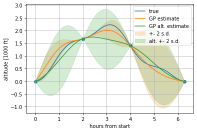
Comparison of estimated altitudes with samples of the derivatives (GP estimate in orange) and without samples of the derivatives (GP alt. estimate in green).

We can see that the orange line follows the blue line more closely than the green. Additionally, we can see the impact of the samples of the derivatives in the uncertainty of each estimate. The shaded areas give the estimate ± two standard deviations. This uncertainty of the estimate stays low around the two-hour mark, because the method not only knows the value at that time, but how Harvey was moving at the time as well. Further away from the derivative samples the effect disappears, as can be seen in the region between the four-hour and six-hour marks where the two estimates are similar.

In other cases, adding samples of the derivative can be used to force a point to be modelled a local maximum, and this is how I first encountered the concept. But as the example shows, the idea is much more general than that.

Footnotes

1. The covariance function expresses our assumptions on the form of the function. For instance, the squared exponential covariance function drops off radially with distance. Other choices could e.g. introduce a periodic structure. Several covariance functions are visualised here.
2. Assuming that the covariance function is differentiable.
3. By limiting ourselves to a single feature dimension we simplify the notation, but the concepts extend to multi-dimensional features.

References

[1] Rasmussen, C. E. and Williams, C. K. I. (2006) Gaussian Processes for Machine Learning. MIT Press.

Aug 31, 2020

Derivatives and Gaussian Processes / CDT Data Science Blog by blogadmin is licensed under a Creative Commons Attribution CC BY 3.0

Research, Tutorials

What are Gaussian Processes?

An example

Now add derivatives

Continuing our example

Footnotes

References

Share

Leave a Reply Cancel reply

Report this page