Day 1 – The Morning and Halfway up

Friday 3rd March from 6am – 10:30am

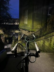
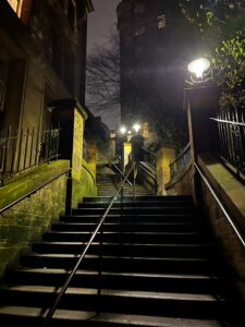
Waking up bright and early at 5am for a 6am field recording at the steps – the city was quiet, dark, and peaceful… if you don’t count listening to all the delivery trucks and bin lorries.

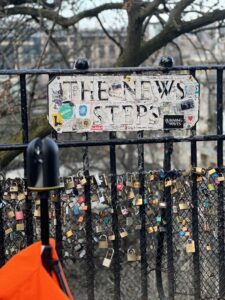
We arrived at The New Steps with an ok-ish attitude, a considerable amount of caffeine, and a plan, to record the scans for the first section of the steps. Deciding to start from the bottom of the steps, we set up everything, took out our companion and biggest ally for the day our buddy Liam the LiDAR (yes we named him, it was a long day), and hit record.

The initial plan was to take one scan on every landing of the steps, just changing the scanner to the right or to the left after each one. But after the first couple of tries, we discovered that we were missing quite a lot of information from the middle of the steps, making the scans look quite empty.

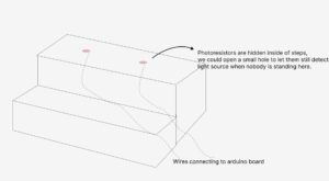
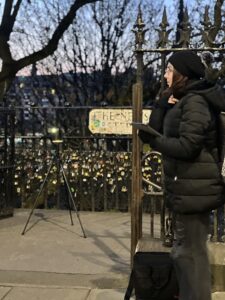
So very carefully we adjusted one of the legs of the tripod and placed the scanner in the middle space between the landings. Because we know how expensive the scanner is, and we were really afraid of someone walking down the steps in a rush and accidentally kicking it, Molly took the role of bodyguard, sitting down right under the scanner to make sure it will stay in its place. And in some scans you can see a bit of blue flashing right next to where the scan was placed, this was the top of Molly’s hat peeking thru.

Around our sixth scan, the iPad showed 10% of the battery left, and the storage was completely full, making us unable to keep scanning.  So we went looking for somewhere to charge the electronics, and to warm up for a bit as well. We ended up in the New College where The School of Divinity is located. Asking at the main entrance where we could sit and work for a bit, we headed to Rainy Hall, and settled down there, to export the scans from the iPad into our external hard drive, and then import them to Cyclone.

Here was when we realized just how much data we had gathered so far, as we could not export the bundle from the iPad because we had no storage in it, so we had to export each file individually, then delete it, over and over. Once we had all the files, we put them into Cyclone, and manually aligned each and every single scan, and when we were ready to export them so we could move to CloudCompare, we could not. Why? because the laptop also had no memory left (just our luck).

So back to the steps we went to finish scanning the four places we were missing. And once we were done with it, we waited for the sound team to finish their recordings, and we all headed to Alison House to finish processing the data. Once in the Atrium, we exported the rest of the scans and added them to the bundle in Cyclone. After a bit of trial and error, we were finally able to connect our external hard drive to Cyclone and export our first bundle of scans, yey!

The overall experience for this first day of fieldwork was quite nice, as once we had the scans all together and were able to see just how much amazing data we gathered during some hours in the morning, it made us excited to keep working and looking forward to experimenting with it.

Day 2 – The Afternoon/Evening and the Second Half

Tuesday 7th March from 1:30pm – 7pm

One would have thought that going out at 5am in the morning would be way harder than doing the same thing during the middle of the day, but boy we were wrong. It was much colder this day, making it extremely hard for us to feel comfortable standing on the steps while doing the scans.

We did the first batch of scans from 1pm to around 3pm as we wanted to record the mid-day rush, we quickly notices just how much more movement the was on the steps, as there were quite a good amount of tourists going up and down. We knew that they were tourists because once they hit the middle of the steps, they all looked lost and tried to go thru the gates that lead somewhere else, thinking it was the exit because that is what google maps tells you to go. So we kindly acted as guides telling them that they still had to go up another big stretch of stairs.

We went to charge the iPad and then came back around 4pm to do a couple of scans for the evening part. Then we needed to wait until the sun was setting, so we went to find refuge from the cold in a coffee shop. This day felt like it was neverending, we were sitting down drinking our coffees looking at the window waiting for the sun to go down and it would just not do it. It wants until about 6:30 pm that we could see the sky changing, so we ran back to the stairs and did the final part of it. And just like that, we were done with all our scans. We still had to go and process the data and join the two bundles together, but this was way easier than the first time we did it.

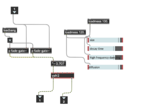
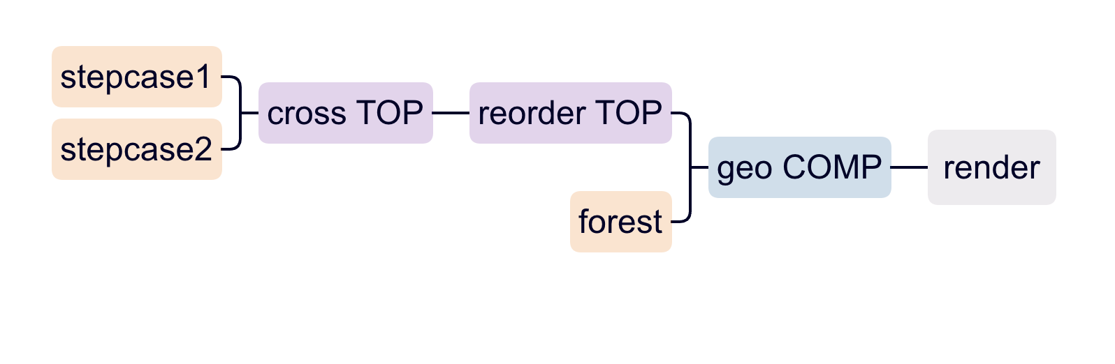
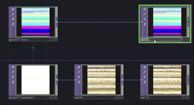
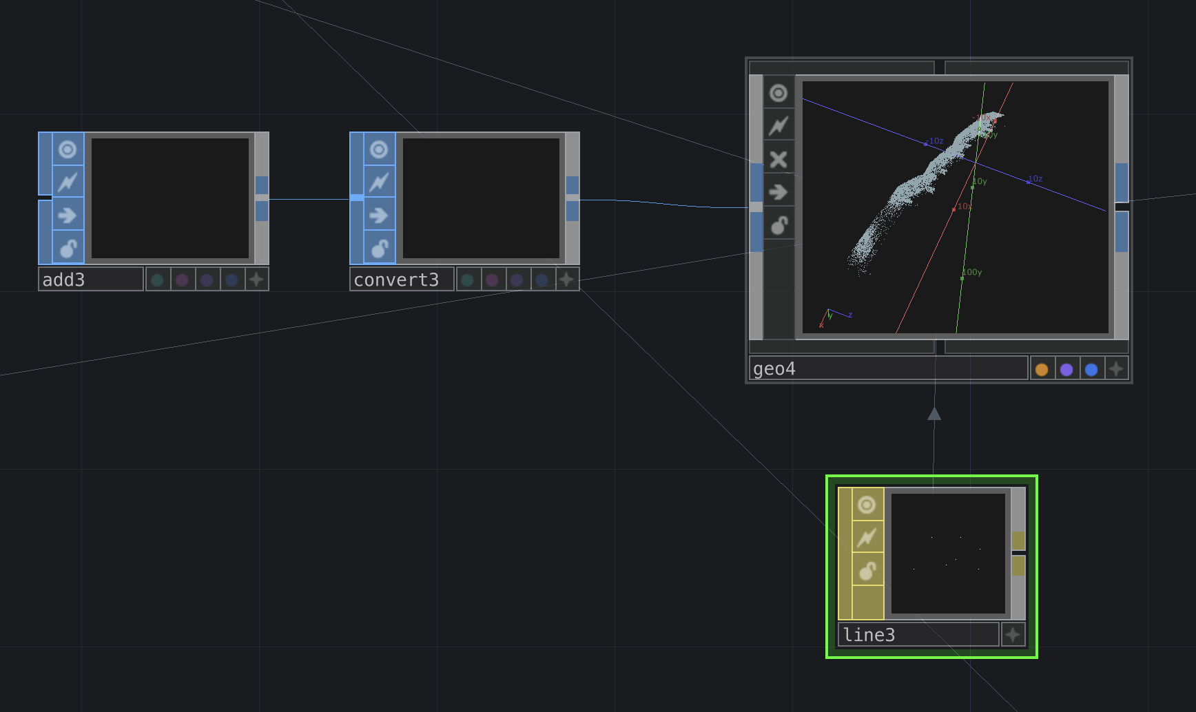
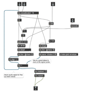
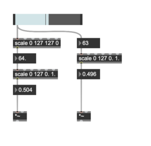
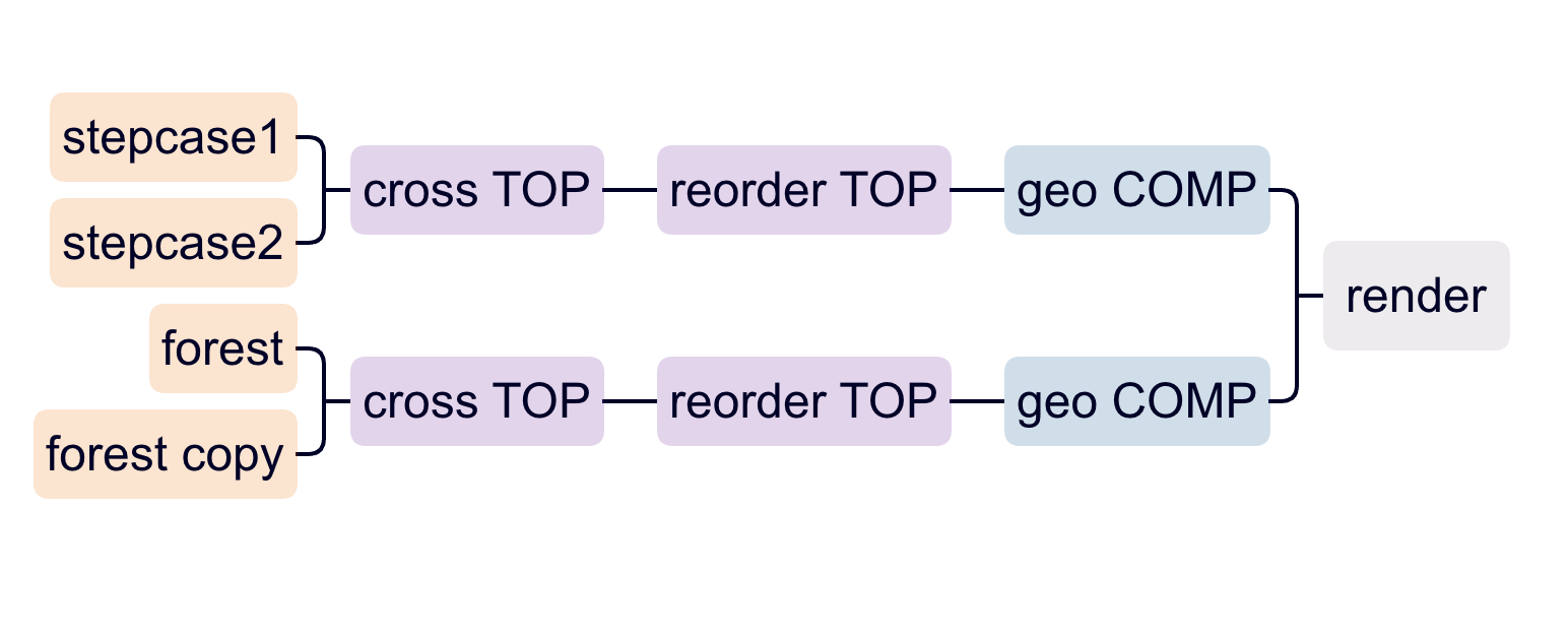
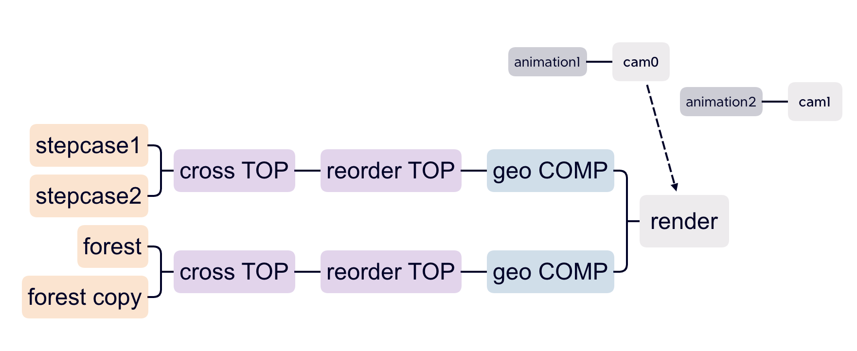
We knew we had gathered a huge amount of data, but I don’t think we were ready when we did the math and found out we had more than one billion points. So it really makes sense why our computers sounded like they were dying while we were processing the data. After some subsampling of our cloud point, we created different versions of it, some to use in blender, unity, or touch designer, and some for our sound teammates to process using MaxMSP.

Timetable

Scan	Location	Time
1	Bottom gate	7 AM
2	Bottom stairs base	7:13
3	Flight 1 mid	7:30
4	Landing 1	7:42
5	Flight 2 mid	8am
6	Landing 2	8:10
7	Flight 3 mid	10am
8	Landing 3	10:11
9	Flight 4 mid	10:22
10	Landing 5	10:30
11	Flight 4 mid	1:30 PM
12	Landing 5	2
13	Flight 5 mid	2:10
14	Landing 6	2:20
15	Flight 6 mid	2:25
16	Landing 7	2:43
17	Flight 7 mid	2:48
18	Landing 8 top	4:40
19	Top tip top outside	4:45
20	Flight 7 mid	6:30
21	Landing 8top 2	6:40

If you’re reading this in order, please proceed to the next post: ‘Field Recording Report’.

Molly and Daniela

Mar 23, 2023

After discussing with Yijun and Allison, we decided to prepare two sets of camera animations for the two scenes respectively. In addition, we designed interaction for Scene 2 by using Kinect to recognize the user’s hands. To ensure that the content of Scene 2 does not affect Scene 1, the forest section also needs to be duplicated and correspond to Scene 1 and Scene 2 separately. This also allows for more freedom in interactive design, as we can individually control the changes, colors, and interactions of the staircase and forest sections in each scene.

Rendering structure

To implement the above ideas, we decided to redesign the rendering structure of the scene. We used two Geo TOP to display the staircase and forest sections separately and used Cross TOP and Reorder TOP to synchronize switching between the two staircase scenes and the two forest scenes. With this setup, when the values of the two Cross TOPs are both 0, the rendered content will be Scene 1. When both Cross TOPs receive a value of 1, the two sections switch simultaneously, and Scene 2 is rendered.

Camera switching

To synchronize the two different camera animations with the scene switching, I decided to use two cameras and create animations for them separately. I referred to Ruben(2021)’s tutorial on TouchDesigner multi-camera switching on YouTube. To switch between the cameras, an expression was set in the camera parameters in the Render TOP: ‘cam{0}’.format(int(op(‘null16’)[‘chan2’])). By receiving values of 0-1 similar to the Cross TOP, the floating point number is converted to an integer through int(), which switches the view between the two cameras cam0 and cam1.

 

If you’re reading this in order, please proceed to the next post: ‘TouchDesigner Point Cloud Camera Animation#1’.

 

 

Yuxuan Guo

Mar 22, 2023

Ambient sound, as one of the most intuitive feelings when people are in a “place”, is a very important attribute of the “place” itself. In order to present this property in our installation, we decided to go to the selected location “The News Steps” for field recording to record the ambient sound, edit and process it as one of the elements of the installation sound design, and deliver it to David for sonification in max/msp and to Xiaoqing for interactive sound design.

 

Because our installation is time-related, we wanted to be able to record the entire day from morning to night, and the duration of the recording would be very long. At the same time, “The News Steps” is a public outdoor space, which poses additional challenges for field recording and requires thorough preparation.

 

Before making the equipment list, I went to “The News Step” for a site survey. It is a steep and very narrow staircase, but fortunately, there are some small platforms in the middle of the large section of stairs for us to set up the equipment. The pedestrians here are dense and of all ages, so during the recording process, one is to protect the equipment from harm, and the other is to observe the pedestrians’ reactions to the equipment before the formal recording. If they can ignore them and present the most natural way is the best, if they have surprised, curious and funny reactions is also acceptable. The most worrying situation is that people will shut up because they notice the microphones, making the walkers feel disturbed or even offended, which would completely defeat the purpose of recording the daily sound of the place and is something we definitely don’t want to see. If this happens during the test recording, we will reduce the use of microphones that are more familiar to passersby (e.g., shotgun mics). We were initially concerned that such recordings would violate some rights such as the privacy of pedestrians, but since we will do some processing so that the final presentation does not show the original voice or content, so there should be no such risk.

The list of equipment that I have drawn up, taking into account various considerations, can be found in the blog linked below.

https://blogs.ed.ac.uk/dmsp-place23/wp-admin/post.php?post=421&action=edit

After discussing this with the group, we decided to simplify the list to two pairs of condenser mics and a shotgun mic, which was more than enough to represent the ambient sound of the location. In addition to the recording equipment itself, I included batteries, tape, and a large-capacity SD card in the list to prepare for long recording times and various other issues that might arise. Here is the link to the first sound meeting.

https://blogs.ed.ac.uk/dmsp-place23/wp-admin/post.php?post=388&action=edit

 

We took the equipment to “The News Steps” for a test recording before the formal recording, found the appropriate platform to set up the system, created the work area, smoothly adjusted the equipment and started recording. Two pairs of microphones(Neumann KM184 pair and Shcoeps MK6 pairs) were recorded at fixed locations using the mixpre6II, while the shotgun mic(Sennheiser MKH 416) was recorded using h6 to flexibly roaming around the stairs. The test recording proved to be very necessary. Although we prepared a large number of batteries, the weather was so cold, especially for the mixpre6II, that four brand-new AA batteries would not even last 15 minutes. In addition, since the recording scene was outdoors, the low-frequency noise brought by the wind would be very serious and affect the overall effect if there were no windproof measures. Unfortunately, we had to record the next day and it was too late to use the bookit to borrow some windshields. So we found everything we could use in an emergency to put over the microphone, including a little plush hat that came with the purchase of a drink. Because these things are not so tight for the microphone, I found in the monitoring when the wind is relatively strong, there was the sound of friction between them and the mics.  So we used tape to fix them a bit and finally solved the problem. It was a very moving and fun experience for me to see everyone working together to solve a problem. The good news is that the recorded sound was very good and the passersby hardly reacted to the microphone, which made me determined to continue using the shotgun mic.

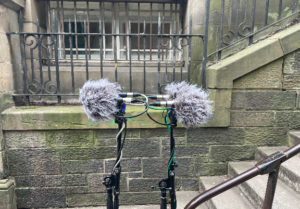
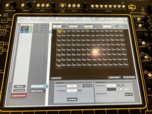
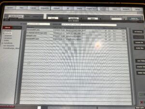
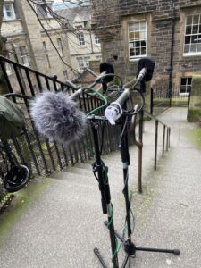
After the test recording, I tested it again at home and exported the recording from the SD card to check. Because the mixpre6II’s advance working mode is used, the sound is recorded as poly-wave. Because two pairs of microphones are used, the file has six tracks, the first two tracks are a stereo mix of all microphones, and the last four tracks are separate signals from each of the four microphones. In this way, as long as I recorded the input channel number for each microphone, I could easily tell which microphone was recording the current signal in post-editing. After checking, since our two pairs of microphones were placed back-to-back, the recorded signal did not have phase problems and the mixed signal from the first two tracks could be used directly (provided that the balance of each track was adjusted during recording). There was another unexpected gain in the process: if the recorder was powered through the computer, it would last much longer than four AA batteries. But I couldn’t rule out at the time that it was because the room was warmer, so I still brought an extra H6 recorder as plan b when I was formal recording.

On the first formal recording day, the group woke up at 5 am and met at “The News Steps” at 6 am to set up the system. (It was really cold!) Because of the experience of the trial recording, the process went very smoothly. The computer was connected to power the recorder and the input channels for each microphone were recorded. Because of problems with the time code inside the recorder, I specifically recorded the duration, start time and end time of each recording. I expected the length of each strip to be ten minutes after editing, so I kept each recording at about 15 minutes. After David’s reminder, I would say the exact time to the microphone at the beginning of each recording, so it would be easier to edit. It was very touching that all the sound design students participated in this field recording with such an early start time and a long duration. The team worked very well together. After setting up the system, some students stayed here to record and monitor, while others helped to buy breakfast. After that, the recording also alternated in turns, with me mainly controlling the mixpre6II and monitoring the two pairs of main microphones, while the other three alternated using the shotgun mic for more flexible recording. In addition to recording the sounds made by pedestrians, they also recorded their own footsteps, the sounds of the environment around the steps, their own chats with passersby, the barking of dogs on the roadside, and other very interesting sounds in preparation for the production of interactive sounds later, all in an orderly manner. As time went on, we also changed the position of the main microphone pairs once, placing them on a higher platform to accommodate the “the higher you go, the later it gets” concept of our installation. Fortunately, the computer’s battery held up until the recording was successfully completed. More photos and details can be found in the blog at the link below.

https://blogs.ed.ac.uk/dmsp-place23/wp-admin/post.php?post=442&action=edit

https://blogs.ed.ac.uk/dmsp-place23/wp-admin/post.php?post=450&action=edit

After that, I started to edit the recorded sound. Since there was still a problem with wind noise in the low end, I did a slight dynamic EQ on it, which solved the problem very effectively. At the same time, I went through the edit from the beginning, cutting out any excessive low-end wind noise and other unwanted sounds, and keeping each strip to exactly 10 minutes (for David’s sonification later). Because the final installation will have a large number of channels, in addition to all mixed together in stereo, I also rendered two pairs of microphones each in stereo and four microphones each in mono, naming them fixedly in the time_microphone_L/R/stereo format for easy handover.

The second recording was for the afternoon to evening period. I borrowed four windshields of the same type to try to avoid the problem of low-frequency wind noise, and thanks to them, they helped us to protect these very delicate microphones from the sudden heavy snowfall. Luckily the snow only lasted for a short while and the rest of the recording was not much different from the first time, as we had previous experience and overall it went very well.

Currently, I have finished editing the field recording and delivered the data to the students in the follow-up session. I have learned a lot and the group has become more familiar and united with each other, which is a very new and wonderful experience for me. Afterwards, I will be working with the sound design team to do follow-up work and working with Allison to see if we can combine Max and Kinect to trigger some sounds through audience movement.

Here are the Google drive link of the edited audio files:

March 03

https://drive.google.com/file/d/1JuxCVSa_C8AAwWZ3-oHS88mH-ewmU5fN/view?usp=share_link

March 07

https://drive.google.com/file/d/13BwTmicp3CXq94gKffz5gaxBcPhxRSFv/view?usp=share_link

 

If you’re reading this in order, please proceed to the next post: ‘Arduino 1st Stage’.

Chenyu Li

 

Mar 19, 2023

The previous post documented what can be seen as the beginning sound block of the sonification piece, which replicates the same sonified granular system across the eight channels of a 7.1 surround system, each crossfading to a second on triggered for interactive audio replacement. By this stage, the sounding result is a texture with spectral qualities that feel similar to the high-fidelity soundscape capture but granularly rearranged, providing a first sense of acceptance and normality, followed by disorientation and pattern unrecognition when listening actively—a result of the interest of its own, and presented in the final result as such. However, further resynthesis and processing were desired, a linear variable that could morph between this first scenario and one other that felt otherworldly, hollow, and with an “upside down” feeling. This linear variable was achieved by designing a parallel crossfaded signal flow, with heavy processing between a delay line loop and a parallel reverb. This “morphing linear variable” was envisioned with the intent of interfacing with user-controlled gestures that will be explored in further blog posts.

A delay system can be achieved in Max/MSP by simply using a ~tapin and a ~tapout together, where the very common “Delay Time” parameter is defined through this second one. These two objects, on their own, however, do not sound “delayed” in the sense of the effect. Since these two objects delay an incoming signal once, no repetition of this instance will be heard. Therefore, and as commonly known across the common conception of a delay effect, a signal loop is built into this system with a signal multiplier factor between the value of 0 and 1, which as a variable is famously known as the “Feedback Amount”. With the feedback loop set, the signal gets re-delayed to silence like an expected “traditional” delay effect, and from this point, things get more interesting. By allocating other types of processing inside this loop, the effects will also get repeated accordingly. When these processing block’s parameters behave dynamically, things get really interesting. This way, we no longer solely loop an audio signal but also the effect of the processing blocks over time. In this project, three processing blocks are set, with there respective parameters:

• • A low-pass filter — Cut-off frequency;
  • A pitch shifter — Pitch;
  • And a tremolo/ring-modulator — Modulating frequency and Ramp Time;

Having this set-up settled, this dynamic behaviour that shapes sound in such interesting ways is provided by the method of sonification by assigning the fluctuations of the variable by the flowing data set and its factors (previously described in the past blog posts). After some experimentation and careful tuning over scale a smoothening, the sonification reflects over the following connections:

• • Delay Time –> R coordinate;
  • Feedback Amount –> Intensity; 
  • Cutoff Frequency –> G coordinate;
  • Pitch –> B coordinate;
  • Tremolo/Ring -Modulation modulator frequency –> X coordinate
  • Ramp time Tremolo/Ring -Modulation –> Y coordinate.

Another processing aspect of this parallel path in a crossfaded linear variable is a reverb unit inspired by the Cycle’74 example. With a fixed set of parameters, this reverb unit presents a very large, reflective-sounding place with a hollow and industrial feel. (Figure 1)

As the last blog post mentioned, this system is set individually across each of the eight channels of the 7.1 surround sound system.

If you’re reading this in order, please proceed to the next post: ‘Sonfication #5 – 7.1 Panning and Surround Sound Layout’.

Mar 19, 2023

Building on our previous work with Arduino sensors, we’ve decided to switch to an ultrasonic sensor based on the feedback from our recent lecture. For safety reasons, we won’t be creating physical steps for our exhibition. Instead, we’ll utilize a distance sensor to detect audience movement and trigger video swapping.

 

Figure.1. Screenshots of code

 

Expanding Our Horizons

Figure.2. Screenshots of  the max patch

To collaborate effectively with our sound designer team, we’ve also explored connecting Arduino sensors with MAX/MSP. It’s been exciting to learn something new and understand how serial ports can be displayed in various forms. The key takeaway is that the central concepts remain the same: using the same port and converting data into a format MAX can understand.

Challenge & ChatGPT

During our development process, we encountered a few hiccups. The data we received from the Arduino monitor differed from what appeared in the Processing console. After double-checking the circuit, Arduino code, and port, we turned to ChatGPT for help.

As it turned out, we hadn’t converted the string data to an integer or removed any leading/trailing whitespace. ChatGPT provided a solution that fixed our issue perfectly!

Figure.3. My lovely online tutor

What’s Next?

Our next step is to experiment with the speed() and jump() functions in Processing to explore the possibilities of controlling a single video’s playback speed or direction. Ideally, the video would play faster and faster as the audience approaches the sensor.

Stay tuned for more updates as we continue refining our interactive experience!

If you’re reading this in order, please proceed to the next post: ‘Arduino 3rd stage – Connecting to Touchdesigner!’.

 

Allison Mu

03/16/2023

Mar 16, 2023

We’re excited to dive into the world of Arduino sensor testing! Our goal is to create an interactive experience where different videos play when our audience steps on a physical model of new steps. To accomplish this, we’ve chosen a particular sensor that’s both easy to attach and discreetly hidden beneath the steps.

Selecting the Ideal Sensor

After some consideration, we decided on using a photoresistor due to its ease of attachment and perfect size for hiding below the steps. Check out our ideal sensor implementation in Figure 1 below:

Figure.1. Ideal sensor implementation for the steps

 

Devices

• Arduino Uno R3
• Photoresistor
• 220-ohm resistor
• Jump wires
• breadboard

Software

• Arduino IDE
• Processing

 

Figure.2&3. Screenshots of the code

 

Integrating Video Playback

Since Arduino doesn’t have its own video library, we need to link it with another coding program, such as Python, MAX/MSP, or Processing, to achieve the desired result. The logic behind this is using a serial port to transfer data from Arduino to Processing, and setting up two thresholds to switch between the recorded videos.

While these codes aren’t overly complex, they provide valuable insight into sharing Arduino data with other software. As a team, our long-term plan is to connect sensors with Unity or Touch Designer to directly manipulate the movement of the camera. However, it’s always smart to have a backup plan (e.g., video swapping) for the exhibition.

Stay tuned for more updates on our Arduino sensor testing journey!

 

Lets see how it works!

https://www.youtube.com/shorts/SvZ2pgWlxWo

 

If you’re reading this in order, please proceed to the next post: ‘Arduino 2nd Stage’.

 

Allison Mu

02/16/2023

Mar 16, 2023

Previously, I mentioned that I divided the original point cloud data into three parts: Staircase 1, Staircase 2, and Forest. Now, we want to make Scene 1 and Scene 2 change interactively while keeping the forest section fixed. 

To make the transition between the two scenes natural, I used the Cross TOP and Reorder TOP to implement the transition by scrambling the points in one scene and then re-generating the second scene. This method was inspired by the TDSW(2022). Additionally, I can use the Noise TOP to add noise to each axis individually to achieve changes in the point cloud in a specific direction.

When transitioning between scenes, the parameter range for Cross TOP is from 0 to 1. When the value is 0, the content of Scene 1 is displayed, and when the value is 1, the content of Scene 2 is displayed. The middle part of the range between 0 and 1 represents the transition process between the two scenes.

The specific idea is to use a distance sensor to detect the position of the audience, set two distance intervals, and map the values of these two intervals to the range of 0-1 in TouchDesigner. When the user is close to the sensor, Scene 1 is displayed, and when the user moves back to a distance further from the sensor, Scene 2 is displayed.

 

Yuxuan Guo

Mar 15, 2023

To transfer point cloud files to TouchDesigner for further editing, we referred to the videos uploaded by B2BK(2023) and Heckmann(2019) on YouTube as a reference.

Separating coordinates and colors.

 In TouchDesigner, we used the pointfilein TOP to import point cloud files in the PLY format that were previously exported. Afterward, we used the pointfileselect TOP to separate the corresponding color sections in the point cloud file. The colour values are encoded from 0 to 127 in the ply file. To get the right colours, it’s necessary to create a math TOP and divide by 127.

Adding materials.

Next, we created a Geometry COMP and added an Add SOP and Convert SOP to it. Then, we linked the point cloud coordinates and colors from the previous steps in the Geometry COMP. Then, we added a Line MAT as the material for the Geometry COMP, and the basic point cloud import operation was complete.

Rendering

Finally, to display the point cloud, we needed to add a Render TOP to render the contents of the Geometry COMP. The Render TOP also needs to be used in conjunction with a Camera COMP and a Light COMP for proper rendering.

In addition to these steps, we can also use the Point Transform TOP to adjust the position of the point cloud in 3D space, and use tools such as the Ramp TOP to adjust the color of the point cloud during the first step.

 

If you’re reading this in order, please proceed to the next post: ‘Touchdesigner visual part 1 – import point cloud file into touchdesigner #2’.

Yuxuan Guo & Yijun Zhou

Mar 11, 2023

The audio team met with Roderick on 3 March to discuss how to achieve 7.1 surround sound. With Roderick’s help, the audio team was introduced to the use and setup of the SD11 Mixer.

I have designed two surround sound plans for this purpose and the audio team will finalise the plans after sound testing.

Mar 6, 2023