Summary of the Kolmogorov-Obukhov (1941) theory: overview.
Summary of the Kolmogorov-Obukhov (1941) theory: overview.
In the last three posts we have summarised various aspects of the Kolmogorov-Obukhov (1941) theory. When considering this theory, the following things need to be borne in mind.
[a] Whether we are working in $x$-space or $k$-space matters. See my posts of 8 April and 15 April 2021 for a concise general discussion.
[b] In $x$-space the equation of motion (NSE) simply presents us with the problem of an insoluble, nonlinear partial differential equation.
[c] In $k$-space the NSE presents a problem in statistical physics and in itself tells us much about the transfer and dissipation of turbulent kinetic energy.
[d] The Karman-Howarth equation is a local energy balance that holds for any particular value of the distance $r$ between two measuring points.
[e] There is no energy flux between different values of $r$; or, alternatively, through scale.
[f] The energy flux $\Pi(k)$ is derived from the Lin equation (i.e. in wavenumber space) and cannot be applied in $x$-space.
[g] The maximum value of the energy flux, $\Pi_{max}=\varepsilon_T$ (say), is a number, not a function, and can be used (like the dissipation $\varepsilon$) in both $k$-space and $x$-space.
[h] It also matters whether the isotropic turbulence we are considering is stationary or decaying in time.
[g] If the turbulence is decaying in time, then K41B relies on Kolmogorov’s hypothesis of local stationarity. It has been pointed out in a previous post (Part 2 of the present series) that this cannot be the case by virtue of restriction to a range of scales nor in the limit of infinite Reynolds number [1]. See also the supplemental material for [2].
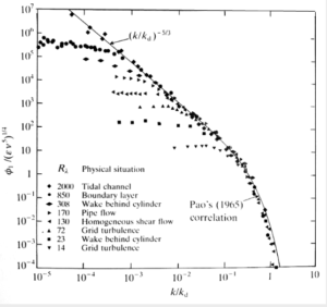
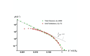
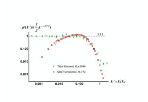
[h] In $k$-space this is not a problem and the $k^{-5/3}$ spectrum can still be expected [1], as of course is found in practice.
[i] If the turbulence is stationary, then K41B is exact for a range of wavenumbers for sufficiently large Reynolds numbers. The extent of this inertial range increases with increasing Reynolds numbers.
I have not said anything in this series about the concept of intermittency corrections or anomalous exponents. This topic has been dealt with in various blogs and soon will be again.
[1] W. D. McComb and R. B. Fairhurst. The dimensionless dissipation rate and the Kolmogorov (1941) hypothesis of local stationarity in freely decaying isotropic turbulence. J. Math. Phys., 59:073103, 2018.
[2] W. David McComb, Arjun Berera, Matthew Salewski, and Sam R. Yoffe. Taylor’s (1935) dissipation surrogate reinterpreted. Phys. Fluids, 22:61704, 2010.