Is it possible to achieve an infinite Reynolds number?
There has been an increasing awareness in the turbulence community of the significance of finite-Reynolds-number (FRN) effects, corresponding to an impression that Kolmogorov’s theory requires an infinite Reynolds number. At the same time, there has been a recent growth of interest in Onsager’s Conjecture, which is essentially taken to mean that turbulent dissipation is still present even when the Reynolds number is infinite, and this is normally interpreted as being when the fluid viscosity is zero. Oddly, there never seems to be any mention of the word ‘limit’; and one detects a degree of uncertainty about the whole matter, with typical comments like: ‘when the Reynolds number is infinite, or at least very large’.

In order to examine this topic, we may begin by remarking that the Newtonian fluids we study always have a finite viscosity. Also, reducing the viscosity seems like an unlikely method of increasing the Reynolds number. If we take pipe flow as an example, the normal procedure is to increase the velocity of the fluid, as being much easier than increasing the pipe diameter or decreasing the fluid viscosity. Nevertheless, the idea of varying the viscosity has been around for a long time, with Batchelor discussing the idea of taking the limit as $\nu \rightarrow 0$, at a constant rate of dissipation. He argued that this would push the effect of viscosity to an infinite value of the wavenumber, i.e. $k=\infty$ [1]. Edwards took the idea further; and, in order to test his statistical theory, argued that the input (due to forces) and the output (due to viscosity) could be represented by delta functions at $k=0$ and $k=\infty$, respectively [2]. However, both examples were in the context of continuum mechanics and, most importantly, involved the taking of limits. That is, the case of $\nu=0$ is the Euler equation, and there is no dissipation. The case $\nu \rightarrow 0$, such that dissipation is maintained constant, involves a limiting process and is the Navier-Stokes equation in the infinite Reynolds limit. It is not the Euler equation.

This procedure of taking the viscosity to tend to zero can seem counter-intuitive; but an example that is even more so can be found in microscopic physics, where the classical limit can be obtained by letting Planck’s constant $h$ tend to zero. This is definitely counter-intuitive: after all, $h$ is not just a constant, it is a universal constant. The answer to this is that we must be taking a limit where the quantum levels become infinitesimally small in comparison to the energies involved in the macroscopic system.

We can apply the same idea to turbulence. For pipe flow, we can work with a non-dimensional viscosity of the form $\tilde{\nu}=\nu/U d$, where $U$ is the bulk mean velocity and $d$ is the diameter of the pipe. Evidently increasing the velocity is the equivalent of decreasing the scaled viscosity. Moreover, as the scaled velocity is a pure number, concepts of large and small are better defined.

The idea of zero scaled viscosity then corresponds to an infinite value of the velocity and clearly is not achievable. So, in practice, zero scaled viscosity means that it is small enough compared to other relevant quantities that it may be neglected. The best way to do this, is to look for a limit. That is, as the scaled viscosity tends to zero, the dissipation (say) tends asymptotically to a constant value. When variations in the dissipation are too small to resolve, either numerically or experimentally, we have in fact reached a limiting value. This behaviour can be seen in the variation of dissipation rate with increasing Reynolds number in reference [3].

[1] G. K. Batchelor. The theory of homogeneous turbulence. Cambridge University Press, Cambridge, 2nd edition, 1971. (First published 1953).
[2] S. F. Edwards. Turbulence in hydrodynamics and plasma physics. In Proc. Int. Conf. on Plasma Physics, Trieste, page 595. IAEA, 1965.
[3] W. D. McComb, A. Berera, S. R. Yoffe, and M. F. Linkmann. Energy transfer and dissipation in forced isotropic turbulence. Phys. Rev. E, 91:043013, 2015.

Postscript. This is my first post in some time because I have been busy with acting as Guest Editor in a special edition of Atmosphere. I hope to post frequently from now on. The link to the journal is:
https://www.mdpi.com/journal/atmosphere/special_issues/FOH7AK5UB1

 

 

Special Issue of the journal Atmosphere on Isotropic Turbulence.

It has been some time since I last posted, and the title of this post suggests the main reason, as being a Guest Editor has proved to be quite time consuming. Nevertheless, I have agreed to be Guest Editor because, although I think it is a rather ambitious project, I also believe that it is very timely.

The Special Issue has the subtitle Recent Advances and Current Challenges, and further details can be found at the link:

https://www.mdpi.com/journal/atmosphere/special_issues/FOH7AK5UB1

Our aim in this Special Issue is to publish papers which can help to identify the most recent advances and what the current challenges are. Hence, we are asking for submissions that have both a pedagogical and a review perspective.

At the moment, I am writing an Editorial to give an overview of the subject and to try to indicate some promising candidates for being regarded as significant advances. Equally, I hope to be able to suggest some topics which can be classified as current challenges.

We already have six promised contributions and two have been posted on the website as tentative titles; and I hope that many more will contribute to this worthy attempt to clear up some long-standing issues in the study of isotropic turbulence. The submission deadline is 29 February 2024. You may send your manuscript now or up until the deadline. Submitted papers should not be under consideration for publication elsewhere. The journal also encourages authors to send a short abstract or tentative title to the Editorial Office in advance (atmosphere@mdpi.com). Further details of how to submit to this Open Access journal may be found at the link for the special issue.

If anyone would like to discuss their ideas for a possible paper with me, I will be very happy to hear from them.

 

 

Two-time correlations and temporal spectra: the analysis by Tennekes [1].
In this post we take a closer look at the analysis by Tennekes [1] in which he differed from the earlier analysis of Tennekes and Lumley [2] and concluded that large-scale sweeping is the determining factor in the decorrelation of the two-time correlation in the inertial range. As noted in my post of 27 April 2023, this leads (rather confusingly) to a `$-5/3$’ power law for the Eulerian temporal spectrum, when the Kolmogorov form is actually $n=-2$. His starting point is equation (1) in [1], which may be written in our present notation as: \begin{equation}\frac{\partial u_1}{\partial t}=-\left(u_1\frac{\partial u_1}{\partial x_1}+u_2\frac{\partial u_1}{\partial x_2}+u_3\frac{\partial u_1}{\partial x_3}\right),\end{equation} and this is justified by assuming that Taylor’s hypothesis of frozen convection applies.

The usual application of Taylor’s hyopothesis is to situations where there is a mean or free stream velocity $U_1$, which is much larger than the turbulent velocity $\mathbf{u}(\mathbf{x},t)$. Then the changes in the velocity field with time at a fixed measuring point could be due to the passage of a frozen pattern of turbulent motion past that point. Hence the local time derivative at a point may be replaced by the convective derivative, thus: \begin{equation}\frac{\partial}{\partial t} \rightarrow -U_1\frac{\partial}{\partial x_1} \quad \mbox{if} \quad U_1 \gg u.\end{equation} Or in the context of spectra, \begin{equation}k_1 = \omega/U_1.\end{equation} A fuller discussion of this can be found in Section 2.6.5 of [3].

Thus (1) seems a rather extreme application of Taylor’s hypothesis. In fact we can write down an exact expression for ${\partial u_1}/{\partial t}$ by invoking the Navier-Stokes equation. This gives us \begin{equation}\frac{\partial u_1}{\partial t}=-\left(u_1\frac{\partial u_1}{\partial x_1}+u_2\frac{\partial u_1}{\partial x_2}+u_3\frac{\partial u_1}{\partial x_3}\right)-\frac{\partial p}{\partial x_1} + \nu \nabla^2 u_1,\end{equation} where $p$ is the kinematic pressure and $\nu$ is the kinematic viscosity. Thus in using equation (1), Tennekes neglects both the pressure and the viscous terms. The latter may seem reasonable, as his main concern was with the inertial range, but it must be borne in mind that the subsequent analysis involves squaring and averaging both sides of equation (1) so the neglect of the viscous term may introduce significant error. However, the neglect of the pressure term is even more concerning, as this is a highly non-local term with the pressure being expressed in terms of integrals of functions of the velocity field over the entire system volume: see Section 2.1 of [3].

This analysis relies on imponderable assumptions about scale separation and statistical independence. Such ideas were discussed much later on, and rather more quantitatively, in the context of mode eliminations and large eddy simulation: see Chapter 8 in the book [4] for an account of this work. It is clear that the analysis by Tennekes has swept a great deal under the carpet. In contrast, the arguments given by Tennekes and Lumley [2] seem, to me at least, more confident and well justified than those given in [1]. In his conclusion, Tennekes remarked on the difference between the two analyses, stating that it was `embarrassing in a personal sense.’ Certainly both sets of arguments might repay closer study.

As a final point, he expresses the view that the implications of [1] support Kraichnan’s view that Lagrangian coordinates are more suited to statistical closure theories than the more usual Eulerian variety. However, it is worth pointing out that all the analyses that support such a view are valid (if at all) only for stationary turbulence, whereas all the numerical assessments of closure theories are restricted to freely decaying turbulence. I intend to go on working on this topic as time permits.

[1] H. Tennekes. Eulerian and Lagrangian time microscales in isotropic turbulence. J. Fluid Mech., 87:561, 1975.

[2] H. Tennekes and J. L. Lumley. A first course in turbulence. MIT Press. Cambridge, Mass., 1972.

[3] W. D. McComb. The Physics of Fluid Turbulence. Oxford University Press,
1990.

[4] W. David McComb. Homogeneous, Isotropic Turbulence: Phenomenology,
Renormalization and Statistical Closures. Oxford University Press, 2014.

Two-time correlations and temporal spectra: the Lagrangian case.
In my previous post on 27 April 2023, I promised to come back to the Lagrangian case. Over the years, I have taken the view that the discussion of the Lagrangian case along with the Eulerian case, which is the one that is of more practical importance, is an unnecessary complication. At the same time, I have had to acknowledge that the application of these ideas to the assessment of statistical closure theories should take account of the fact that there are Lagrangian theories as well as Eulerian theories. However, there is an interesting point to be made when we compare the treatment in the book by Tennekes and Lumley [1] with the later analysis of Tennekes [2].

In the previous post, we only mentioned the discussion by Tennekes and Lumley [1] of the inertial range behaviour of the Eulerian spectrum. In fact they not only derive the inertial range form of the Lagrangian spectrum, and find it to be the same power law as the Eulerian case, but also obtain a relationship between the constants of proportionality in the two cases.

The crucial step in this work is the equivalence of the two correlations (see Section 8.5 of [1]), where the authors refer back to their discussion of Lagrangian forms in Section 7.1 (actually they incorrectly give this as 7.2). Following their notation, we represent the Lagrangian velocity of a fluid point by $V_{\alpha}(t)$ where $\alpha = 1, 2, \mbox{or}, 3$. Then, they assert that $\langle V_{\alpha}V_{\alpha}\rangle =\langle u_{\alpha} u_{\alpha}\rangle$, where $u_{\alpha}$ is of course the Eulerian velocity; leading on to their equation (8.5.3). This is the step that provides the basis for their assertion of the equivalence of the Eulerian and Lagrangian inertial range spectra.

However, the later work of Tennekes [2] leads to the Eulerian spectrum being different from the Lagrangian form, due to the supposed predominance of sweeping effects. This would seem to be an inconsistency and we will return to this in future posts when we examine the work of Tennekes more closely.

We close by pointing out that in our previous post we noted that the form of two-time correlation being studied in [1] was limited to stationary flows. This point was also made by Hinze [3]: see equation (1.57), page 39 in the first edition. However, in discussing the motion of fluid points in Lagrangian coordinates, Tennekes and Lumley emphasise the need for both homogeneity and stationarity. So in effect this restriction has already been made. We also note that an alternative discussion of the original work by Lumley can be found in Section 12.2 of [4].

[1] H. Tennekes and J. L. Lumley. A first course in turbulence. MIT Press. Cambridge, Mass., 1972.
[2] H. Tennekes. Eulerian and Lagrangian time microscales in isotropic turbulence. J. Fluid Mech., 87:561, 1975.

[3] J. O. Hinze. Turbulence. McGraw-Hill, New York, 1st edition, 1959.

[4] W. D. McComb. The Physics of Fluid Turbulence. Oxford University Press,
1990.

Two-time correlations and temporal spectra
I previously discussed this topic in my posts of 25 February 2021 and 10 March 2022. In the succeeding months I have become increasingly aware that there is dissension in the literature, with people citing the temporal spectrum as $\omega^{-2}$, if the arguments of Kolmogorov apply; and $\omega^{-5/3}$, if convective sweeping applies. Statements about these forms are often made without any supporting reference, so my next step was to identify the sources; and then try to make a critical assessment of both forms and their relationship to each other. In fact the source of the first result seems to be the book by Tennekes and Lumley [1], while the second form is due to later work by Tennekes [2]. So here I will make a start by outlining the general problem, in order to fix notation and definitions.

We begin with the general two-point, two-time correlation tensor $R_{\alpha\beta}(\mathbf{x},\mathbf{x’};t,t’)$, where $\alpha$ and $\beta$ are the cartesian tensor indices, taking the values $1,2$ or $3$. The correlation is defined in terms of the velocity field $u(\mathbf{x},t)$, thus: \begin{equation}R_{\alpha\beta}(\mathbf{x},\mathbf{x’};t,t’)=\langle u_\alpha(\mathbf{x},t)u_\beta(\mathbf{x’},t’)\rangle, \end{equation} where the angle brackets denote the ensemble average. In everything that follows we will restrict our attention to homogeneous turbulence and consider a fixed point in space. This means that we may simplify the notation by omitting the space variables, and write the correlation tensor as: \begin{equation}R_{\alpha\beta}(\mathbf{x},\mathbf{x’};t,t’)=R_{\alpha\beta}(t,t’). \end{equation} Then, for generality, we may introduce the sum and difference variables for the times, as: \begin{equation} \mathcal{T}=(t+t’)/2 \quad \mbox{and} \quad \tau = (t’-t). \end{equation} Accordingly, the two-time correlation tensor may be written in the form: \begin{equation} R_{\alpha\beta}(t,t’) = R_{\alpha\beta}(\mathcal{T},\tau) \end{equation} We still have one more restriction to make: Tennekes and Lumley restrict their attention to isotropic turbulence, which means that we can replace the correlation tensor by a single scalar correlation function which we will denote by $R_E$, where the subscript $E$ denotes `Eulerian’. Thus, for isotropic turbulence, \begin{equation}R_{\alpha\beta}(\mathcal{T},\tau) \rightarrow R_E(\mathcal{T},\tau), \end{equation} In a later post we will introduce the Lagrangian correlation function.

Now, at this stage, we have imposed all the restrictions that Tennkekes and Lumley have made in specifying their problem. However their subsequent analysis seems to imply that they are also considering stationary turbulence and this is an important point. We will underline this fact by continuing to treat the problem more generally.

The energy spectrum $\phi_E(\mathcal{T},\omega)$ is defined by the Fourier transform, \begin{equation}R_E(\mathcal{T},\tau) = \int_{-\infty}^\infty \exp(i\omega \tau) \phi_E(\mathcal{T},\omega)d\omega,\end{equation}where $\omega$ is the angular frequency; and the Fourier pair is completed by: \begin{equation}\phi_E(\mathcal{T},\omega)= \frac{1}{2\pi}\int_{-\infty}^\infty \exp(-i\omega \tau)R_E(\mathcal{T},\tau)d\tau.\end{equation}

As a preliminary to considering the inertial-range form of $\phi_E(\mathcal{T},\omega)$ we need to establish its dimensions. If we integrate the spectrum over all frequencies, we have: \begin{equation} \int_{-\infty}^{\infty}\phi_E(\mathcal{T},\omega)d\omega = U^2(\mathcal{T}),\end{equation} where $U$ is the root mean square velocity. Recall that $\mathcal{T}$ is the clock time, as opposed to the difference time $\tau$. From this relationship it follows that the dimensions of the spectrum are: \begin{equation} [\phi_E(\mathcal{T},\omega)] = L^2 T^{-1}, \end{equation} where as usual square brackets indicate the dimensions of a quantity.

At this point we assume stationarity, which is in effect what Tennekes and Lumley have done [1] and we omit the dependence on $\mathcal{T}$. Having, in effect, done this, they apply the well known argument of Kolmogorov to limit the dependence of the spectrum to the two independent variables $\omega$ and the dissipation rate $\varepsilon$. They state that the only dimensionally consistent result is: \begin{equation} \phi_E(\omega) \equiv f(\varepsilon, \omega) = \beta \varepsilon \omega^{-2},\end{equation} where $f$ is some arbitrary function, assumed to be a power and $\beta$ is a constant. Checking the dimensions, we find: \begin{equation} [\phi_E(\omega)] = (L^2 T^{-3})T^{2} = L^2 T^{-1}, \end{equation} as required.

Later Tennekes presented a different analysis [2] in which he argued that the inertial-range temporal spectrum would be determined by convective sweeping and this led to the result: \begin{equation}\phi_E(\omega)= \beta_E \varepsilon^{2/3}U^{2/3}\omega^{-5/3}. \end{equation} It is readily verified that this result has the correct dimensions, thus: \begin{equation} [\phi_E(\omega)] = (L^2T^{-1})^{2/3}(LT^{-1})^{2/3}T^{5/3}= L^2T^{-1}.\end{equation}
It should be noted that irrespective of the merits or otherwise of this analysis by Tennekes, it is limited to stationary turbulence in principle due to omission of any dependence on the clock time $\mathcal{T}$. In future posts I intend to give some critical attention to both these theories.

[1] H. Tennekes and J. L. Lumley. A first course in turbulence. MIT Press. Cambridge, Mass., 1972.
[2] H. Tennekes. Eulerian and Lagrangian time microscales in isotropic turbulence. J. Fluid Mech., 87:561, 1975.

Mode elimination: taking the phases into account: 5

When I began this series of posts on the effects of phase, I had quite forgotten that I had once looked into the effects of phase in quite a specific way. This only came back to me when I was using my own book [1] to remind me about conditional averaging. And that book was published as recently as 2014!

In effect, McMillan and Ferziger tested the significance of taking phase into account as long ago as 1979, in the context of sub-grid modelling [2]. They did this by measuring correlations between exact sub-grid stresses and eddy viscosity models. In the case of the Smagorinsky model, which is widely used with reasonable success in shear flows, they found correlations as low as 0.1 – 0.2. Then, in 1998, McComb and Young [3] showed that, for isotropic turbulence at least, low values of the correlations between sub-grid stresses and eddy-viscosity models are due to phase effects. A brief pedagogical demonstration of the need to take phases into account in an eddy-viscosity model can be found in Section 8.7 of [1], but we will not pursue that here; but instead concentrate on the numerical demonstration of the effects of phase.

We carried out a numerical simulation of stationary, isotropic turbulence, with the velocity field in wavenumber defined on the interval $0\leq k \leq k_0$. Various cut-off wave numbers $k_1 \leq k_0$, $k_2 \leq k_1$, $k_3 \leq k_2$; and so on, were considered, so that a series of large-eddy simulations could be compared to the fully resolved simulation. I discussed in my post of 23 March 2023 how the complex velocity field in wavenumber (a.k.a the Fourier transform of the real-space velocity field) could be separated into amplitude and phase; and this was the method employed in [3], from which I have taken three figures. In all cases, we evaluated a correlation coefficient $R(k)$ and this is plotted against $k/k_$, where $k_1$ is the maximum resolved wavenumber in all cases.

In Figure A, we show the correlation $R(k)$ between the subgrid stresses and the eddy viscosity for seven cut-off wavenumbers in the range $16.5 \leq k_1 \leq 112.5$ with $k_0 = 128$. It can be seen that for most cases (shown by continuous lines) the correlation is not very good, varying from $0.25 – 0.5$ at the cut-off wavenumber to essentially being anti-correlated as $h/k_1 \rightarrow 0$. The exceptions are the curves for the lowest cut-off wavenumbers $k_1 =16.5$ (long dashes) and $k_1= 32.5$ (short dashes); and in particular the first of these. It should be noted that the first of these is the only one to yield a finite plateau region in the plot of the effective viscosity against wavenumber [3]. This latter property is an indication that it is only this lowest cut-off wavenumber which gives an adequate degree of scale separation compared to the maximum value.

FIG A

In Figure B, we show the phase correlations for the same cases, and the similarity to the results of Figure A are quite marked.

FIG B

On the other hand, the results for amplitude correlations in Figure C show a high level of correlation over the entire range of wavenumbers, with very little variation between the results for the various cut-off wavenumbers.

FIG C

In this case, isotropic turbulence, we are mainly interested in modelling the inertial transfer through wavenumber and for this purpose a model which represents the amplitudes is quite effective. However, given that all such formulations are based on average quantities it is not easy to see how the phases can be taken into account.

[1] W. David McComb. Homogeneous, Isotropic Turbulence: Phenomenology, Renormalization and Statistical Closures. Oxford University Press, 2014.
[2] O. J. McMillan and J. H. Ferziger. Direct testing of subgrid-scale models. AIAA Journal, 17:1340, 1979.
[3] W. D. McComb and A. J. Young. Explicit-Scales Projections of the Partitioned Nonlinear Term in Direct Numerical Simulation of the Navier-Stokes Equation. Presented at 2nd Monte Verita Colloquium on Fundamental Problematic Issues in Turbulence: available at arXiv:physics/9806029 v1, 1998.

Mode elimination: taking the phases into account: 4

In the previous post we came to the unsurprising conclusion that as a matter of rigorous mathematics, we cannot average out the high-wavenumber modes while leaving the low-wavenumber modes unaffected. However, turbulence is a matter of physics rather than pure mathematics and the initial conditions are not known with mathematical precision. Here the concept of deterministic chaos comes to our rescue. If we accept that the initial condition must have some uncertainty attached to it, then there is a possibility that such an average can be carried out approximately.

We can generalise the conditional average, given as equation (3) in the previous post, by extending it to some arbitrary well-behaved functional $H[u(k,t)]$. Here we are also using the simplified notation of the previous post; and in fact we shall simplify it even further, and write $u(k,t)\equiv u_k$. Then we can replace that equation by:\begin{equation}\langle H[u_k]\rangle_c = \langle H[u_k]\mid u^-_k \rangle,\end{equation} where, as before, the subscript `$c$’ on the left hand side denotes `conditional average’; and the notation on the right hand side indicates that the ensemble average is carried out while keeping the low-wavenumber part of the velocity field $ u^-_k$ constant. From the previous discussion, we know that this average amounts to a delta function, as both $u_k$ and $u^+_k$ are also held constant.

The way out of this impasse is the recognition that, in the real physical situation, $u^-_k$ cannot be held precisely to any exact value. There must be some uncertainty, however small, in the application of this constraint. Accordingly we introduce an uncertainty into our definition of a conditional average by writing it as: \begin{equation}\langle H[u_k]\rangle_c = \langle H[u_k]\mid u^-_k + \phi^-_k\rangle.\end{equation} Evidentally, $ u^-_k + \phi^-_k$ must be a solution of the Navier-Stokes equation, but the uncertainty $\phi^-_k$ is otherwise arbitrary and may be chosen to have convenient properties. In fact, McComb, Roberts and Watt [1] chose it to satisfy the conditions:\begin{equation} \langle u^-_k\rangle_c = u^-_k + \langle \phi^-_k \rangle_c,\end{equation} along with:\begin{equation} \langle u^-_k u^-_j\rangle_c = u^-_k + \langle \phi^-_k \phi^-_j \rangle_c,\end{equation} and \begin{equation} \langle u^-_ku^+_j\rangle_c = u^-_k \langle u^+_k \rangle_c.\end{equation} These relationships are then used in decomposing the NSE and implementing an RGl calculation. It should be noted that $ \langle u^+_k \rangle_c$ is not zero and an equation of motion must be derived for it.

The problem posed by the correction terms in $\phi^-_k$ depends on just how chaotic the turbulence is, but the calculations suggest that these terms can be neglected. In fact the calculation of the invariant energy flux yields a value of the Kolmogorov spectral constant of $\alpha = 1.62$ which is the generally accepted value. Further details can be found in the original paper [1] and in the appropriate sections of the book [2].

However, despite the above procedures, there are still phase effects that are not being taken into account, and this will be the subject of the next post.

[1] W. D. McComb, W. Roberts, and A. G. Watt. Conditional-averaging procedure for problems with mode-mode coupling. Phys. Rev. A, 45(6):3507- 3515, 1992.
[2] W. David McComb. Homogeneous, Isotropic Turbulence: Phenomenology, Renormalization and Statistical Closures. Oxford University Press, 2014.

 

Mode elimination: taking the phases into account: 3

In this post we look at some of the fundamental problems involved in taking a conditional average over the high-wavenumber modes, while leaving the low-wavenumber modes unaffected.

Let us consider isotropic, stationary turbulence, with a velocity field in wavenumber space which is defined on $0\leq k \leq k_0$. Note that the maximum wavenumber $k_0$ is not the Kolmogorov dissipation wavenumber, although in both large-eddy simulation and in the application of renormalisation group (RG) to turbulence, it is often taken to be so. The only definition that I know of, is the one I put forward in 1986 [1], which is:\begin{equation}\int^{k_0}_0 2\nu_0 k^2 E(k)dk \approx \int^{\infty}_0 2 \nu_0 k^2 E(k)dk = \varepsilon, \end{equation} where $\nu_0$ is the kinematic viscosity of the fluid, $E(k)$ is the energy spectrum, and $\varepsilon$ is the dissipation rate. Obviously the value of $k_0$ depends on how closely the integral on the left approximates the actual dissipation rate, which corresponds to the upper limit on the integral being taken as infinity. Some people apparently find this definition puzzling, possibly because they are familiar with RG in the context of the theory of critical phenomena, where the maximum wavenumber is determined by the inverse of the lattice constant. In contrast, fluid dynamicists may find our definition here quite intuitive, as it is analogous to Prandtl’s definition of the laminar boundary layer.

Something which may be counter-intuitive for many, is the choice of $k_0$ as the maximum wavenumber. This is because in RG we progressively eliminate modes in wavenumber bands: $k_1\leq k \leq k_0$, $k_2 \leq k \leq k_1$, $k_3\leq k \leq k_2$, and so on, where $k_n$ decreases with increasing integer $n$, until the iteration reaches a fixed point. Also, the fluid viscosity $\nu_0$ is so denoted, because it is progressively renormalized until it reaches a value $\nu_{n-1}=\nu_n \equiv \nu_N$, at the fixed point $n=N$.

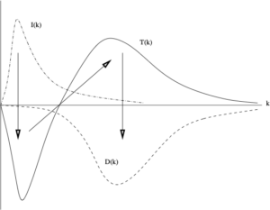
The first step in eliminating a band of modes is quite straightforward. We high-pass, and low-pass, filter the velocity field at $k=k_1$, thus: \begin{eqnarray} u^{-}(k,t) = u(k,t) \quad \mbox{for} \quad 0 \leq k \leq k_1; \nonumber\\ u^{+} (k,t)= u(k,t) \quad \mbox{for} \quad k_1 \leq k \leq k_2,\end{eqnarray} where we have adopted a simplified notation. Then we can substitute the decomposition given by equation (2) into the Navier-Stokes equation in wavenumber, and study the effect. However we will not pursue that here, and further details can be found in Section 5.1.1 of [2]. Instead, we will concentrate here on the following question: how do we average out the effect of the $u^+$ modes, while keeping the $u^-$ modes constant?

The condition for such an average can be written as: \begin{equation}\langle u^-(k,t)\rangle_c = u^{-}(k,t),\end{equation}where the subscript `$c$’ denotes `conditional’. We should also recall that isotropic turbulence requires a zero mean velocity, that is: $\langle u(k,t)\rangle=0$.

Actually, it would be quite simple to carry out such an average, provided that the velocity field $u(k,t)$ were multivariate normal. In that case, each of the various modes could be averaged out, independently of all the rest. However, the turbulent velocity field is not Gaussian so, in attempting to carry out a such an average, we would run into the following two problems.

First, we must satisfy the boundary condition between the two regions of $k$-space. Hence, \begin{equation} u^-(k_1,t)=u^+(k_1,t). \end{equation} This is the extreme case, where we would be trying to average out a high-$k$ mode while leaving the identical low-$k$ mode unaffected. At the very least, this draws attention to the need for scale separation.

Secondly, there are some questions about the nature of the averaging over modes, in terms of the averaging of the velocity field in real space. In order to consider this, let us introduce a combined Fourier transform and filter $F_T^{\pm}(k,x;t)$ acting on the velocity field $u(x,t)$, such that:\begin{equation}u^{\pm}(k,t)=F_T^{\pm}(k,x;t)u(x,t). \end{equation} Noting that both the Fourier transform and the filter are purely deterministic entities, the average can only act on the real-space velocity field, leading to zero!

So it seems that a simple filtered average, as used in various attempts at subgrid modelling or RG applied to turbulence, cannot be correct at a fundamental level. We will see in the next post how the introduction of a particular kind of conditional average led to a more satisfactory situation [3].

[1] W. D. McComb. Application of Renormalization Group methods to the subgrid modelling problem. In U. Schumann and R. Friedrich, editors, Direct and Large Eddy Simulation of Turbulence, pages 67- 81. Vieweg, 1986.
[2] W. David McComb. Homogeneous, Isotropic Turbulence: Phenomenology, Renormalization and Statistical Closures. Oxford University Press, 2014.
[3] W. D. McComb, W. Roberts, and A. G. Watt. Conditional-averaging procedure for problems with mode-mode coupling. Phys. Rev. A, 45(6):3507- 3515, 1992.

 

Mode elimination: taking the phases into account: 2

In last week’s post, we mentioned Saffman’s criticism of models like Heisenberg’s theory of the energy spectrum in terms of their failure to take the phases into account. In this post we explore this idea and try to elucidate this criticism a little further. We can take Heisenberg’s model as representative and an introductory discussion of it can be found in Section 2.8.1 of reference [1]. It is also discussed in Batchelor’s book, and he made the general comment about it: `The notion that the small eddies act as an effective viscosity is plausible enough but does not seem a suitable description of the mutual action of eddies whose sizes are of the same order of magnitude.’

In other words, he is expressing the need for what later became known as `scale separation’: see, for example Section 5.1.1 of the book [3]. (Note: in last week’s post I incorrectly wrote scale invariance when I meant scale separation. This has now been corrected.)

This is an important observation, and it is related to the way in which the phases come into the problem; but Batchelor did not mention this particular aspect. However, if we wish to be precise about the concept of phase, then we must turn again to Batchelor’s book [2], where on page 83 he remarked that the Fourier components of the velocity field are complex, and hence may be written, in the usual way, in terms of an amplitude and a phase. In other words, for any particular wavenumber and time, $u_\alpha(\mathbf{k},t)$ is a complex number.

Accordingly, following Batchelor, and with a change of notation, we may write: \begin{equation} u_\alpha(\mathbf{k},t) = |u_\alpha(\mathbf{k},t)| \exp\{i\theta_\alpha(\mathbf{k},t)},\end{equation}where $i = \surd\{-1\}$, $\theta_\alpha$ is the phase, and the Cartesian index $\alpha$ takes the values $\alpha=1,2,3$.

Batchelor then discussed its general importance, remarking that: `The exchanges of energy are dependent, in general, on the relationships between the phases of the different Fourier component as well as on their amplitudes, and it is in the elucidation of the average properties of the phase relations that the key to the determination of the energy spectrum during the decay lies.’

Little more has been said on this aspect of turbulence theory, apart perhaps Kraichnan’s frequent use of the term `phase mixing’ in his many papers on the direct interaction family of closures: for further details see either of the books [1] or [3]. In the next post we will look more specifically at mode elimination to try to establish what the limitations of the process are.

[1] W. D. McComb. The Physics of Fluid Turbulence. Oxford University Press, 1990.
[2] G. K. Batchelor. The theory of homogeneous turbulence. Cambridge University Press, Cambridge, 2nd edition, 1971.
[3] W. David McComb. Homogeneous, Isotropic Turbulence: Phenomenology, Renormalization and Statistical Closures. Oxford University Press, 2014.

 

Mode elimination: taking the phases into account: 1

This is my first blog this year, very largely because I have been working on a review article as my contribution to a journal issue commemorating Jack Herring, who died last year. We were asked to include some personal recollections of Jack, in addition to the physics, and I began by remarking that I had first met Jack Herring at the NASA-ICASE workshop on turbulence theory at Virginia Beach in October 1984. Taking part were physicists, mathematicians and engineers; and I, as very much a new boy, was glad to be welcomed into the physicists’ group with Jack, Bob Kraichnan and various others.

This was a long time ago, and I only have a few memories of the social interactions, but I do recall that there was a `No-host cocktail hour’ when the day’s programme finished. I was quite amused by this phrase, which I hadn’t met before, and which simply meant that the organisers weren’t about to pay for the drinks! Thinking about this reminded me of an interaction with Phillip Saffman, which I think leads to a point of general interest.

My purpose at the workshop was to give a talk on my application of renormalization group (RG) to turbulence and details of that, along with the other talks may be found in the published proceedings [1]. I do not recall much discussion after the talks but I do remember that Philip Saffman stood up when questions were invited after my talk. He pointed out that my method wouldn’t work because I hadn’t taken the phase into account! When I joined him at the `No host cocktail hour’, he said that he hoped that I didn’t mind his comment. I assured him that I didn’t as I had no idea what it meant. We didn’t discuss it further, and spoke of other matters; but it was to act as the grit in the oyster which ultimately leads (one hopes) to a pearl.

At the time I was uneasy about my theory anyway, and began to play safe and classify it as a mean-field theory. After some years of brooding about this, and other things, I saw that eliminating modes from the Navier-Stokes equation, while leaving other modes unaffected, required a nontrivial conditional average. I worked on this with two of my students, and we formulated a conditional average, along with a means of approximating it, which led to a better theory: see references [2]-[4] and also see [5]

However, in recent years I was reading some lecture notes by Saffman from the sixties [6], and I saw that he had made a similar criticism of theories such as that of Heisenberg (see Section 2.8 of the book [7]), which represented the effect on lower wavenumbers of inertial transfer to higher wavenumbers by some model. In Heisenberg’s case, this involved an eddy viscosity hypothesis, but Saffman made the general criticism of all models of this type, which ran as follows.

`Conceptually, the theories are also objectionable as they ignore the phases of the Fourier components and almost regard Fourier components as having a real physical existence, rather than being a mathematical representation of the motion.’

He doesn’t explain any further what he means by this, nor does he mention the lack of scale separation of the kind that justifies the calculation of the viscosity in the kinetic theory of gases. I will return to these points in the next blog post, but what really fascinates me is the cultural dissonance, which seems to take us into the realm of the philosophy of science. This too, I hope to return to in a future post.

[1] W. D. McComb. Renormalization Group Methods and Turbulence. In D. L. Dwoyer, M. Y. Hussaini, and R. G. Voigt, editors, Theoretical Approaches to Turbulence. Springer Verlag, 1985.
[2] W. D. McComb and A. G. Watt. Conditional averaging procedure for the elimination of the small-scale modes from incompressible fluid turbulence at high Reynolds numbers. Phys. Rev. Lett., 65(26):3281-3284, 1990.
[3] W. D. McComb, W. Roberts, and A. G. Watt. Conditional-averaging procedure for problems with mode-mode coupling. Phys. Rev. A, 45(6):3507 -3515, 1992.
[4] W. D. McComb and A. G. Watt. Two-field theory of incompressible-fluid turbulence. Phys. Rev. A, 46(8):4797- 4812, 1992
[5] W. D. McComb. Asymptotic freedom, non-Gaussian perturbation theory, and the application of renormalization group theory to isotropic turbulence. Phys. Rev. E, 73:26303-26307, 2006.
[6] P. G. Saffman. Lectures on homogeneous turbulence. In N. Zabusky, editor, Topics in nonlinear physics, pages 485-614. Springer-Verlag, 1968.
[7] W. D. McComb. The Physics of Fluid Turbulence. Oxford University Press, 1990.

 

What are the first and second laws of turbulence?

Occasionally I still see references in the literature to the Zeroth Law of Turbulence. The existence of a zeroth law would seem to imply that there is at least a first law as well. But, so far as I know, there are no other laws of turbulence, and hence my question is purely rhetorical.

The so-called zeroth law is the fact the turbulent dissipation tends to a limit as the Reynolds number increases. Some people seem to be obsessed by the fact that this is equivalent to a finite dissipation limit as the viscosity tends to zero. Unfortunately, they become hypnotised by the zero viscosity and completely overlook the word `limit’! This becomes translated into `finite turbulent dissipation at zero viscosity’ and is also referred to as the `dissipation anomaly’. If this were true, then it certainly would be anomalous, to say the least. But it isn’t true. Turbulent dissipation is ultimately, like all dissipation in fluid systems, the transformation of macroscopic kinetic energy into heat by the action of viscosity. No viscosity means no dissipation.

I do not wish to become hypnotised myself by this particular manifestation of folklore. I have written about it before in these blogs and will write about it again. Right now I wish to concentrate only on the oddity of the terminology: `zeroth law’. Presumably it has been so named by analogy with the situation in thermodynamics, where the well-established first and second laws were later supplemented by both a third law and a zeroth law. The third law was part of the subject when I took my first degree but the zeroth law wasn’t. It amounts essentially to a definition of temperature that provides a basis for its measurement. I suppose that it became thought to be so fundamental that it really ought to precede the existing first and second laws.

However, if that was the case, then surely it would be better to name it something like `The fundamental principle of thermodynamics’? The trouble with zeroth law is that zero means nothing. That is, when you don’t have any of something, then you have zero.

It is a failure to recognise this that causes confusion about the calendar when a century changes. One needs to realize that there is no `year zero’. Everything is zero to begin with. Then we start counting seconds, minutes, days and 365 days later we have achieved one year which we denote by `1’. When we reach ten years, we have completed a decade, and we can label that year by `10’, with zero fulfilling its mathematical significance by giving us a symbol for `10’. Thus the year 10 is the last year of the decade, the year 100 is last year of the century, and the year 1000 is the last year of the millennium. Thus Year 2000 is the last year of the second millennium and Year 2001 is the first year of the third millennium. (I hope that digression made sense!)

In my view, the use of the term `zeroth law’ is lame in thermodynamics and doubly lame in turbulence, where we do not even have an agreed first law. It also reflects muddled thinking, based very largely on a failure to understand the mathematical concept of a limit, which ends up with the erroneous supposition that the infinite Reynolds number limit corresponds to the Euler equation. This amounts to a failure to recognize that the Euler equation throughout its entire life has been indomitably non-dissipative.

This will be my last blog of this year. I intend to resume posting in the new year. In the meantime, I hope that we shall all have a pleasant holiday.

 

 

The non-Markovian nature of turbulence 9: large-eddy simulation (LES) using closure theories.

In this series of posts we have argued that the three pioneering theories of turbulence (due to Kraichnan, Edwards and Herring, respectively) are all Markovian with respect to wavenumber interactions. Thus, despite their many successful features, the ultimate failure of these theories to give the correct infinite-Reynolds number limit arises from the fact that they cannot reproduce the non-Markovian nature of fluid turbulence. In the immediately preceding post, we drew a distinction between the concept of a process being Markovian in its wavenumber interactions and the `almost-Markovian’ nature of certain single-time theories, where the term `Markovian’ refers to their development with time. In this final post in the series, we may shed some further light on these matters by considering the use of closures to calculate the subgrid viscosity for a large-eddy simulation.

This activity was initiated in 1976 by Kraichnan [1] who considered isotropic turbulence and based his approach on his own test-field model. In fact this publication led to quite a lot of activity by others, although this was generally based on the very similar EDQNM model (see the previous post).

The LES equations for isotropic turbulence can be formulated in wavenumber space by filtering the velocity field at some fixed cut-off wavenumber $k_c$. Then, for the explicit (resolved) wavenumbers $k\leq k_c$, we have the resolved velocity field $u^{<}(\mathbf{k,t})$; while the subgrid field takes the form $u^{>}(\mathbf{k,t})$ for $k_c\leq k$. Then substituting into the Navier-Stokes equations, we obtain separate equations for the low-$k$ and high-$k$, ranges. However, the nonlinear term ensures that the two equations of motion are coupled together. This coupling of explicit and implicit modes is the subgrid modelling problem.

A detailed discussion of these matters may be found in Section 10.3 of the book [2], but here we only wish to sketch out some features of Kraichnan’s approach insofar as they bear on the earlier posts in this series. We may do this schematically in terms of the Lin equation, as follows. Evidentally, corresponding to the explicit modes of the velocity field, we may define an explicit modes energy spectral density $C^{<}(k,t)$, and correspondingly the filtered energy spectrum $E^{<}(k,t) = 4\pi k^2 C^{<}(k,t)$. Accordingly we may write the energy balance for the explicit modes as: \begin{equation}\left(\frac{\partial}{\partial t} + 2\nu k^2 \right)E^{<}(k,t) = T^{<}(k,t) + T^{<>}(k,t),\end{equation} where $T^{<}(k,t)$ is the transfer spectrum for the explicit modes and contains only couplings within these modes; whereas $T^{<>}(k,t)$ contains terms involving the implicit modes. Kraichnan proposed [1] that the second transfer term could be modelled in terms of an effective subgrid viscosity $\nu(k|k_c)$, such that \begin{equation}T^{<>}(k,t) \equiv T(k|k_c) =-2\nu(k|k_c)k^2 E^{<}(k,t),\end{equation} where at the same time he introduced the parametric notation shown.

The point that we wish to highlight here is that in using $T(k|k_c)$ Kraichnan only took the output term into acccount. In fact the input term, even if small, must be included. In fact there are circumstances where it is not small and in general $\nu(k_c|k)$ is not positive definite, nor should it be. Thus, an adherence to the Markovian point of view that underpinned the DIA and the other pioneering closures, leads to an incorrect result. A full discussion of this may by found in Section 10.3 of [2] and on page 394 Kraichnan’s effective viscosity can be found as equation (10.17), while the corrected form with the input term of the transfer spectrum included may be found as a footnote on page 403 of the same reference.

As a corollary here, on page 392 of [2] I have noted that Kraichnan showed that his first lagrangian theory reduced to a Markovian form under certain circumstances. In the case of the LET theory, I know that it is non-Markovian but I had only assumed that was the case for all the Lagrangian theories. So, at least for the first one, it has been shown to be the case.

[1] R. H. Kraichnan. Eddy-viscosity in two and three dimensions. J. Atmos. Sci., 33:1521, 1976.
[2] W. D. McComb. The Physics of Fluid Turbulence. Oxford University Press, 1990.

The non-Markovian nature of turbulence 8: Almost-Markovian models and theories

Previously, in my post of 10 November 2022, I mentioned, purely for completeness, the work of Phythian [1] who presented a self-consistent theory that led to the DIA. The importance of this for Kraichnan was that it also led to a model representation of the DIA and in turn to the development of what he called `almost-Markovian’ theories. Some further discussion of this topic can be found in Section 6.3.2 of the book [2], but here we will concentrate on the general class of almost-Markovian models and theories. My concern here is to draw a distinction between their use of `Markovian’, which refers to evolution in time, and my use in this series of posts, which refers to interactions in wavenumber.

This class consists of the Eddy-damped, Quasi-normal, Markovian (EDQNM) model of Orszag in 1970 [3], the test-field model of Kraichnan in 1971 [4], the modified LET theory of McComb and Kiyani in 2005 [5], and the theory of Bos and Bertoglio in 2006 [6]. Here we follow the example of Kraichnan who described a theory which relied on a specific assumption that involved the introduction of an adjustable constant as a model. In order to illustrate what is going on in this kind of approach, I will discuss the EDQNM in some detail, as follows.

We begin with the quasi-normal expression for the transfer spectrum $T(k)$ from the Lin equation. This is found to be: \begin{eqnarray}T(k,t) & & =8\pi^2\int d^{3}j\,L\left(\mathbf{k},\mathbf{j}\right)\int_{0}^{t}ds\,R_0\left(k;t,s\right)R_0\left(j;t,s\right)R_0\left(\left|\mathbf{k}-\mathbf{j}\right|;t,s\right) \nonumber \\& \times &\left[C\left(j,s\right)C\left(\left|\mathbf{k}-\mathbf{j}\right|,s\right)-C\left(k,s\right)C\left(\left|\mathbf{k}-\mathbf{j}\right|,s\right)\right],\label{KWE2} \end{eqnarray} where the viscous response function is given by \[R_0(k;t,t’)=\exp[-\nu k^2 (t-t’)],\] and the coefficient $L(\mathbf{k,j})$ is defined as: \begin{equation}L(\mathbf{k,j}) = -2M_{\alpha\beta\gamma}(\mathbf{k})M_{\beta\alpha\delta}(\mathbf{j})P_{\gamma\delta}(\mathbf{k-j}),\label{lkj1}\end{equation} and can be evaluated in terms of three scalar variables as \begin{equation}L(\mathbf{k,j}) = -\frac{\left[\mu\left(k^{2}+j^{2}\right)-kj\left(1+2\mu^{2}\right)\right]\left(1-\mu^{2}\right)kj}{k^{2}+j^{2}-2kj\mu},\label{lkj2}\end{equation} where $\mu$ is the cosine of the angle between the vectors $\mathbf{k}$ and $\mathbf{j}$. For further discussion and details see Appendix C of the book [7].

Now Orszag argued that the failure of QN was basically due to the use of the viscous response function, when in fact one would expect that the turbulence interactions would contribute to the response function. Accordingly he proposed a modified response function: \begin{equation}R(k;t,t’)=\exp[-\omega(k)(t-t’)],\end{equation}where $\omega(k)$ is a renormalized inverse modal response time. One may note that this is now becoming the same form as that of the Edwards transfer spectrum, but that it is also ad hoc and thus there is the freedom to choose $\omega(k)$. After some experimentation using dimensional analysis, Orszag chose the form: \begin{equation}\omega(k)=\nu k^2 + g\left[\int_0^k dj j^2 E(j)\right]^{1/2},\end{equation} where the constant $g$ is chosen to give the correct (i.e. experimental) result for the Kolmogorov spectrum. This is the eddy damped part of the model, so replacing $R_0$ by $R$ gives us the EDQN.

Even with the introduction of the damping term, the EDQN model can still lead to negative spectra. This was cured by introducing the Markovian step with respect to time. This rested on the assumption that the characteristic time $[\omega(k) +\omega(j) + \omega(|\mathbf{k-j}|)]^{-1}$ is negligible compared to the evolution time of the products of covariances in the expression for $T(k)$. The equation for the transfer spectrum was Markovianised by replacing the time integral by a memory function $D(k,j;t)$, thus: \begin{equation}T(k,t) =8\pi^2\int d^{3}j\,L\left(\mathbf{k},\mathbf{j}\right) D(k,j;t)\left[C\left(j,s\right)C\left(\left|\mathbf{k}-\mathbf{j}\right|,s\right)-C\left(k,s\right)C\left(\left|\mathbf{k}-\mathbf{j}\right|,s\right)\right],\end{equation} where the memory function is given by \begin{equation}D(k,j;t)= \int_0^t ds \, \exp[\omega(k)+\omega(j)+\omega(|\mathbf{k-j}|)](t-s).\end{equation}This is now the EDQNM model.

When applied to the stationary case, this result for $T(k)$ is identical to the Edwards result, as given in the post of 3 November 2022; but there are crucial differences. The function $\omega(k)$ in the Edwards theory arises from a Markovian theory with respect to wavenumber interactions and is accordingly related to $T(k)$, thus giving the second equation of the closure. In contrast, the function $\omega(k)$ in EDQNM is fixed independently of the transfer spectrum by means of dimensional analysis and accordingly is not Markovian in the sense of the Edwards SCF. It is important to distinguish between the two kinds of Markovianisation.

In our next post, we will conclude this series of posts by discussing how these considerations affect the application of closures to large-eddy simulation.

[1] R. Phythian. Self-consistent perturbation series for stationary homogeneous turbulence. J.Phys.A, 2:181, 1969.
[2] W. D. McComb. The Physics of Fluid Turbulence. Oxford University Press, 1990.
[3] S. A. Orszag. Analytical theories of turbulence. J. Fluid Mech., 41:363, 1970.
[4] R. H. Kraichnan. An almost-Markovian Galilean-invariant turbulence model. J. Fluid Mech., 47:513, 1971.
[5] W. D. McComb and K. Kiyani. Eulerian spectral closures for isotropic turbulence using a time-ordered fluctuation-dissipation relation. Phys. Rev. E, 72:16309{16312, 2005.
[6] W. J. T. Bos and J.-P. Bertoglio. A single-time, two-point closure based on fluid particle displacements. Phys. Fluids, 18:031706, 2006.
[7] W. David McComb. Homogeneous, Isotropic Turbulence: Phenomenology, Renormalization and Statistical Closures. Oxford University Press, 2014.

 

The non-Markovian nature of turbulence 7: non-Markovian closures and the LET theory in particular.

We can sum up the situation regarding the failure of the pioneering closures as follows. Their form of the transfer spectrum $T(k)$, with its division into input and output parts, with the latter being proportional to the amount of energy in mode $k$, is only valid for Markov processes, so it is incompatible with the nature of turbulence which is non-Markovian. It is also incompatible with the phenomenology of turbulence, where the entire $T(k)$ acts as input (or output), depending on the value of $k$, as I pointed out in 1974 [1]. It is worth noting that the first measurement of $T(k)$ was made by Uberoi in 1963 [2], so turbulence phenomenology was in its infancy at the time the first closures were being developed. In later years, numerical experiments based on high-resolution direct numerical simulations, did not bear out the Markovian picture. In particular, we note the investigation by Kuczaj et al [3]. This is in fact the basic flaw in Kraichnan’s DIA and also the SCF theories of Edwards and Herring: the fault lies not in the covariance equations but in the relationship of the response function to them.

As mentioned in the first blog in the present series (posted on 13 October) a response to this problem took, and continues to take, the form of an extension of the DIA approach to Lagrangian coordinates. A consideration of these theories would take us too far away from our present objective although it should be mentioned that they are non-Markovian in that they are not expressible as Master equations. Instead we will concentrate on the LET theory which exposes the underlying physics of the turbulence energy transfer process.

The LET theory was introduced with the hypothesis that $\omega(k)$ is determined by the entire $T(k)$, not just part of it, and can be defined by a local energy balance [1]. It was extended to the two-time case [4] in 1978; and, less heuristically, in subsequent papers by McComb and co-workers: see [5] for a review. Essentially, the two-time LET theory comprises the DIA covariance equations plus the generalized fluctuation-response relation. It may be compared to Herring’s two-time SCF [6] which comprises the DIA response equation, single-time covariance equation and the generalized fluctuation-response equation. It may also be compared directly to DIA in terms of response equations. However, for our present purposes, we will go back to the simplest case, and show how LET arose in relation to the Edwards SCF.

It was argued by McComb [1], that a correct assignment of the system response in terms of $T(k)$ (i.e. `correct’ in the sense of agreeing with the turbulence phenomenology of energy transfer) could lead to a response function which was compatible with K41. This was found to be the case and, citing the form given in [1], we may write for the turbulence viscosity $\nu_T(k)$: \begin{equation} \nu_T(k)= k^{-2}\int_{j\geq k}d^3 j \frac{L(\mathbf{k,j})C(|\mathbf{k j}|)[C(k)-C(j)]}{C(k)[\omega(k)+\omega(j)+\omega(|\mathbf{k-j}|)]},\label{let-visc}\end{equation} where $\omega(k) = \nu_T(k) k^2$. The lower limit on the integral with respect to $j$ arises when we consider the flux through mode $k$. It was used in [1] to justify wavenumber expansions leading to differential forms but is not needed here and can be omitted. The interesting point here is made by rewriting this in terms of the Edwards dynamical friction $r(k)$. From equation (5) in the post on 3 November, rewritten as \[\omega(k)=\nu k^2 + \nu_T(k)k^2 =\nu k^2 + r(k),\] we may rewrite (\ref{let-visc}) as: \begin{equation}\nu_T(k)= r(k) – k^{-2}\int d^3 j \frac{L(\mathbf{k,j})C(|\mathbf{k,j}|)C(j)}{C(k)[\omega(k)+\omega(j)+ \omega(|\mathbf{k-j}|)]}. \label{let-visc-rk}\end{equation}

It was shown [1] that the second term in the LET  response equation  cancelled the divergence in $r(k)$ in the limit of infinite Reynolds number. Hence the term which destroys the Markovian nature of the renormalized perturbation theory is the term which makes the theory compatible with the Kolmogorov $-5/3$ spectrum.

In the next post we will consider the subject of almost-Markovian models, where the term refers to the integrals over time rather than to the energy transfer through wavenumber.

[1] W. D. McComb. A local energy transfer theory of isotropic turbulence. J. Phys. A, 7(5): 632, 1974.
[2] M. S. Uberoi. Energy transfer in isotropic turbulence. Phys. Fluids, 6:1048, 1963.
[3] Arkadiusz K. Kuczaj, Bernard J. Geurts, and W. David McComb. Nonlocal modulation of the energy cascade in broadband-forced turbulence. Phys. Rev. E, 74:16306-16313, 2006.
[4] W. D. McComb. A theory of time dependent, isotropic turbulence. J. Phys. A: Math. Gen., 11(3):613, 1978.
[5] W. D. McComb and S. R. Yoffe. A formal derivation of the local energy transfer (LET) theory of homogeneous turbulence. J. Phys. A: Math. Theor., 50:375501, 2017.
[6] J. R. Herring. Self-consistent field approach to nonstationary turbulence. Phys. Fluids, 9:2106, 1966.

 

The non-Markovian nature of turbulence 6: the assumptions that led to the Edwards theory being Markovian.
Turbulence theories are usually referred to by acronyms e.g. DIA, SCF, ALHDIA, \dots, and so on. Here SCF is Herring’s theory and, to avoid confusion, Herring and Kraichnan referred to the Edwards SCF as EDW [1]. Later on, when I came to write my first book on turbulence [2], I referred to it as EFP, standing for `Edwards-Fokker-Planck’ theory. This seemed appropriate as Edwards was guided by the theory of Brownian motion. But it did not occur to me at the time that the significance of this was that his theory was Markovian with respect to interactions in wavenumber space; nor indeed that a Markovian form was the common denominator in all three of the pioneering Eulerian theories. In recent years, it did occur to me that it was not necessary to be so prescriptive; and if one took a less constrained approach the result was a non-Markovian theory, in fact the LET theory.

Following Edwards [3], we define a model system in terms of a Gaussian distribution $P_0[\mathbf{u}]$, which is chosen such that it is normalised to unity and recovers the exact covariance. That is: \begin{equation}\int \mathcal{D}\mathbf{u} \ P_0[\mathbf{u}] = 1,\end{equation} and \begin{equation}\int \mathcal{D}\mathbf{u} \ P_0[\mathbf{u}]\ u_\mu(\mathbf{k},t) u_\beta(\mathbf{k’},t’) = \langle u_\alpha(\mathbf{k},t) u_\beta(\mathbf{k’},t’)\rangle=\delta(\mathbf{k}+\mathbf{k’})C_{\alpha\beta} \mathbf{k};t,t’) \ ,\end{equation} respectively. Then one solves the Liouville equation for the exact probability distribution in terms of a perturbation series with $ P_0[\mathbf{u}]$ as the zero-order term. We will not go into further details here, as we just want to understand how the Edwards theory was constrained to give a Markovian form.

Equations (1) and (2) introduce the two-time covariance. However, in order to explain the Edwards theory, we will consider the single-time case. Also, for sake of simplicity, we will employ the reduced notation of Herring, as used extensively by Leslie [4] and others (see [2]). In this notation we represent the velocity field by $X_i$, where the index is a combined wave-vector and cartesian tensor index (i.e our $\mathbf{k}$ and $\alpha$). Accordingly, we introduce the Edwards-Fokker-Planck operator as the sum of single-mode operators, in the form: \begin{equation} L_{EFP} = -\omega_i \frac{\partial}{\partial X_i}\left(X_i + \phi_i \frac{\partial}{\partial X_i}\right), \label{efp} \end{equation} where $\omega_i$ is a renormalized eddy decay rate and $\phi_i$ is the covariance of the velocity field, such that \begin{equation} \phi_i =\int_{-\infty}^\infty X_i^2 P(X_i)dX_i, \end{equation} and $P$ is the exact distribution. Then it is readily verified that the model equation: \begin{equation}L_{EFP}P^{(F)} = 0 \end{equation} has the Gaussian solution \begin{equation} P^{(F)} = \frac{e^{ X_i^2/2\phi_i}}{(2\pi\phi_i)^\frac{1}{2}}. \end{equation}

However, it is important to note, and is also readily verified, that a more general form of the operator $L_0$, which is given by \begin{equation} L_0 = H(X_i)\left[X_i + \phi_i \frac{\partial}{\partial X_i}\right],\end{equation} where $H(X_i)$ is an arbitrarily chosen well behaved function, also yields the same Gaussian solution for the zero-order equation: \begin{equation}L_0P_0 =0.\label{base-op}\end{equation} Hence at this stage the operator $L_0$ is not fully determined. Edwards was guided by an analogy with the theory of Brownian motion and in effect made the choice \begin{equation} H(X_i) = -\omega_i \frac{\partial}{\partial X_i}, \end{equation}in order to generate a base operator which could be inverted in terms of an eigenfunction expansion of Hermite polynomials. In this process, the $\{\omega_i\}$ appeared as eigenvalues.

It is this specific choice which over-determines the basic operator which constrained the Edwards theory to be Markovian. More recently it was found that a more minimalist choice, allied to a two-time representation, leads formally to the LET theory [5]. We will consider a more physical basis for the LET theory in the next post.

[1] J. R. Herring and R. H. Kraichnan. Comparison of some approximations for isotropic turbulence Lecture Notes in Physics, volume 12, chapter Statistical Models and Turbulence, page 148. Springer, Berlin, 1972.
[2] W. D. McComb. The Physics of Fluid Turbulence. Oxford University Press, 1990.
[3] S. F. Edwards. The statistical dynamics of homogeneous turbulence. J. Fluid Mech., 18:239, 1964.
[4] D. C. Leslie. Developments in the theory of turbulence. Clarendon Press, Oxford, 1973.
[5] W. D. McComb and S. R. Yoffe. A formal derivation of the local energy transfer (LET) theory of homogeneous turbulence. J. Phys. A: Math. Theor., 50:375501, 2017

 

The non-Markovian nature of turbulence 5: implications for Kraichnan’s DIA and Herring’s SCF

Having shown that the Edwards theory is Markovian, our present task is to show that Kraichnan’s DIA and Herring’s SCF are closely related to the Edwards theory.
However, we should first note that, in the case of the DIA, one can see its Markovian nature by considering its prediction for $T(k,t)$, and this was pointed out by no less a person than Kraichnan himself in 1959 [1]. We may quote the relevant passage as follows:

‘The net flow is the resultant of these absorption and
emission terms. It will be noticed that in contrast to the
absorption term, the emission terms are proportional to $E(k)$. This
indicates that the energy exchange acts to maintain equilibrium. If the
spectrum level were suddenly raised to much higher than the equilibrium
value in a narrow neighbourhood of $k$, the emission terms would be
greatly increased while the absorption term would be little affected,
thus energy would be drained from the neighbourhood and equilibrium
re-established. The structure of the emission and absorption terms is
such that we may expect the energy flow to be from strongly to weakly
excited modes, in accord with general statistical mechanical principles.’

Note that the absorption term is what Edwards would call the input to mode $k$ from all other modes, while the emission term is the loss from mode $k$.

Kraichnan’s argument here is essentially a more elaborate version of that due to Edwards, and presents what is very much a Markovian picture of turbulence energy transfer. But, in later years, numerical experiments based on high-resolution direct numerical simulations did not bear that picture out. In particular, we note the investigation by Kuczaj et al [2].

Going back to the relationships between theories, in 1964 Kraichnan [3] showed that if one assumed that the time-correlation and response functions were assumed to take exponential forms (with the same decay parameter $\omega(k,t)$), then the DIA reduced to the Edwards theory, although with only two $\omega$s in the denominator of the equation for $\omega$, rather than the three such parameters as found in the Edwards case: see equations (4) and (5) in the previous blog. Thus the arguments used to demonstrate the Markovian nature of the Edwards theory do not actually work for the single-time stationary form of DIA. See also [4], Section 6.2.6. All we establish by this procedure is that the theories are cognate: that is, they have identical equations for the energy spectrum and similar equations for the response function.

Herring’s SCF has been discussed at some length in Section 6.3 of the book [4]. In time-independent form, it is identical to the DIA with assumed exponential time-dependences. The relationship between the two theories can also be demonstrated for the two-time case. The case for the SCF being classified as Markovian seems strong to me. However, there is some additional evidence from other self-consistent field theories. Balescu and Senatorski [5] actually formulated the problem in terms of a master equation and then treated it perturbatively. Summation of certain classes of diagrams led to the recovery of Herring’s SCF. For completeness, we should also mention the work of Phythian [6], whose self-consistent method resembled those of Edwards and Herring. However his introduction of a infinitesimal response function, like that of DIA, meant that his theory ended up re-deriving the DIA equations.

In the next post we will examine the question of how the Edwards theory came to be Markovian. In particular, we will answer the question: what were the relevant assumptions made by Edwards?

[1] R. H. Kraichnan. The structure of isotropic turbulence at very high Reynolds numbers. J. Fluid Mech., 5:497-543, 1959.
[2] Arkadiusz K. Kuczaj, Bernard J. Geurts, and W. David McComb. Nonlocal modulation of the energy cascade in broadband-forced turbulence. Phys. Rev. E, 74:16306-16313, 2006.
[3] R. H. Kraichnan. Approximations for steady-state isotropic turbulence. Phys. Fluids, 7(8):1163-1168, 1964.
[4] W. David McComb. Homogeneous, Isotropic Turbulence: Phenomenology, Renormalization and Statistical Closures. Oxford University Press, 2014.
[5] R. Balescu and A. Senatorski. A new approach to the theory of fully developed turbulence. Ann.Phys(NY), 58:587, 1970.

[6] R. Phythian. Self-consistent perturbation series for stationary homogeneous
turbulence. J.Phys.A, 2:181, 1969.

 

 

The non-Markovian nature of turbulence 4: the Edwards energy balance as a Master Equation.

In this post we will rely on the book [1] for background material and further details. We begin with the well-known Lin equation for the energy spectrum in freely decaying turbulence, thus: \begin{equation}\label{Lin}\frac{\partial E(k,t)}{\partial t}= T(k,t) – 2\nu k^2 E(k,t),\end{equation} where $T(k,t)$ is the transfer spectum: see [1] for further details. This equation is the Fourier transform of the better known Karman-Howarth equation in real space. But, although the KHE is a local energy balance in the separation of measuring points $r$, the Lin equation is not actually a local energy balance in wavenumber space since the transfer spectrum depends on an integral of the triple-moment over all wavenumbers. For explicit forms, see [1].

The energy spectrum is defined in terms of the covariance in wavenumber space (or spectral density) by the well-known relation: \begin{equation} \label{spect}E(k,t)= 4\pi k^2C(k,t),\end{equation} but in theory it is more usual to work in terms of the latter quantity, and accordingly we transform (\ref{Lin}) into \begin{equation}\label{covlin}\frac{\partial C(k,t)}{\partial t}= \frac{T(k,t)}{4\pi k^2} – 2\nu k^2 C(k,t),\end{equation}.
The Edwards statistical closure for the transfer spectrum may be written as:\begin{equation}\label{sfecov}\frac{T(k,t)}{4\pi k^2}=2\int d^3 j\frac{ L(k,j)C(|\mathbf{k}-\mathbf{j}|,t)\{C(j,t)-C(k,t)\}}{\omega(k,t)+\omega(j,t)+\omega(|\mathbf{k}-\mathbf{j}|,t)},\end{equation} where $L(k,j)=L(j,k)$ and the inverse modal response time is given by: \begin{equation}\label{sferesponse}\omega(k,t)=\nu k^2 + \int d^3 j\frac{ L(k,j)C(|\mathbf{k}-\mathbf{j}|,t)}{\omega(k,t)+\omega(j,t)+\omega(|\mathbf{k}-\mathbf{j}|,t)}.\end{equation} This controls the loss of energy from mode $k$, while the term giving the gain to mode $k$ from all the other modes takes the form: \begin{equation}\label{sfegain}S(k,t)=2\int d^3 j\frac{ L(k,j)C(|\mathbf{k}-\mathbf{j}|,t)C(j,t)}{\omega(k,t)+\omega(j,t)+\omega(|\mathbf{k}-\mathbf{j}|,t)}.\end{equation} Then, the Edwards form for the transfer spectral density may be written as:\begin{equation}\label{sfetrans}\frac{T(k,t)}{4\pi k^2}=S(k,t)-2\omega(k,t)C(k,t),\end{equation} and from (\ref{covlin}) the Edwards theory gives the Lin equation as:\begin{equation}\label{sfecovlin}\frac{\partial C(k,t)}{\partial t}=S(k,t)-2\omega(k,t)C(k,t).\end{equation}

Our next step is to compare this to the Master Equation and for simplicity we will consider a quantum system which can exist in any one of a large number of discrete states $|i\rangle$, where $i$ is a positive integer. The relevant equation is the Fermi master equation (see Section 9.1.2 of the book [2]), which may be written as: \begin{equation}\label{fermi}\frac{d p_i}{d t}= \sum_{j}\nu_{ij} p_j – \left\{\sum_j \nu_{ij}\right\}p_i,\end{equation} where: $p_i$ is the probability of the system being in state $|i\rangle$; $\nu_{ij}$ is the conditional probability per unit time of the system jumping from state $|i\rangle$ to state $|j\rangle$; and the principle of jump rate symmetry gives us $\nu_{ij}=\nu_{ji}$.

Either from this comparison with the Fermi master equation or from comparison with other master equations such as the Boltzmann equation, it is clear that the Edwards theory of turbulence is a Markovian approximation to turbulence which is itself non-Markovian. The two questions which now arise are: first, what are the implications for the other closures due to Kraichnan and to Herring? And, secondly, how did the Markovian nature of the Edwards theory come about? These will be dealt with in the next two posts?

[1] W. David McComb. Homogeneous, Isotropic Turbulence: Phenomenology, Renormalization and Statistical Closures. Oxford University Press, 2014.
[2] W. David McComb. Study Notes for Statistical Physics: A concise, unified overview of the subject. Bookboon, 2014. (Free to download from Bookboon.com)

 

 

The non-Markovian nature of turbulence 3: the Master Equation.

In the previous post we established that the ‘loss’ term in the transport equation depends on the number of particles in the state currently being studied. This followed straightforwardly from our consideration of hard-sphere collisions. Now we want to establish that this is a general consequence of a Markov process, of which the problem of $N$ hard spheres is a particular example.

We follow the treatment given in pages 162-163 of the book [1] and consider the case of Brownian motion, as this is relevant to the Edwards self-consistent field theory of turbulence. We again consider a multipoint joint probability distribution and now consider a continuous variable $X$ which takes on specific values $x_1$ at time $t_1$, $x_2$ at time $t_2$, and in general $x_n$ at time $t_n$; thus; \[f_n(x_1,t_1; x_2,t_2; \dots x_n,t_n).\] We then introduce the conditional probability density: \[p(x_1,t_1|x_2,t_2),\] which is the probability density that $X=x_2$ at $t=t_2$, given that $X$ had the value $X=x_1$ when $t=t_1\leq t_2$. It is defined by the identity: \begin{equation}f_1(x_1,t_1)p(x_1,t_1|x_2,t_2)=f_2(x_1,t_1; x_2,t_2).\label{pdef}\end{equation}

From this equation (see [1]), we can obtain a general relationship between the single-particle probabilities at different times as: \begin{equation}f_1(x_2,t_2)=\int p(x_1,t_1|x_2,t_2)f_1(x_1,t_1)dx_1. \label{pprop}\end{equation}

Next we formally introduce the concept of a Markov process. We now define this in terms of the conditional probabilities. If: \begin{equation}p(x_1,t_1;x_2,t_2; \dots n_{n-1},t_{n-1}|x_n,t_n)=p(n_{n-1},t_{n-1}|x_n,t_n),\label{markdef}\end{equation}then the current step depends only on the immediately preceding step, and not on any other preceding steps. Under these circumstances the process is said to be Markovian.

It follows that the entire hierarchy of probability distributions can be constructed from the single-particle distribution $f_1(x_1,t_1)$ and the transition probability $p(x_1,t_1|x_2,t_2)$. The latter quantity can be shown to satisfy the Chapman-Kolmogorov equation: \begin{equation}p(x_1,t_1|x_3,t_3)=\int p(x_1,t_1|x_2,t_2)p(x_2,t_2|x_3,t_3) dx_2,\label{ck}\end{equation} indicating the transitive property of the transition probability.

It is of interest to consider two specific cases.

First, for a chain which has small steps between events, the integral relation (\ref{ck}) can be turned into a differential equation by expanding the time dependences to first order in Taylor series. Putting $f_1 = f$ for simplicity, we may obtain: \begin{equation}\frac{\partial f(x_2,t_2)}{\partial t}=\int\, dx_1\left\{W(x_1,x_2)f(x_1,t)-W(x_2,x_1)f(x_2,t)\right\}, \label{me}\end{equation} where $W(x_1,x_2)$ is the rate per unit time at which transitions from state $x_1$ to state $x_2$ take place. This is known as the master equation.

Secondly, if $X$ is a continuum variable, we can further derive the Fokker-Planck equation as: \begin{equation} \frac{\partial f(x,t)}{\partial t}= \frac{\partial [A(x)f(x,t)]}{\partial x} + \frac{\frac{1}{2}\partial^2[B(x)f(x,t)]}{\partial x^2}. \label{fp}\end{equation} This equation describes a random walk with diffusivity $B(x)$ and friction damping $A(x)$. A discussion of this equation as applied to Brownian motion may be found on pages 163-164 of [1] but we will not pursue that here.

In the next post we will discuss the Edwards theory of turbulence (and by extension the other pioneering theories of Kraichnan and of Herring) in the context of the present work.

[1] W. D. McComb. The Physics of Fluid Turbulence. Oxford University Press 1990.

 

The non-Markovian nature of turbulence 2: The influence of the kinetic equation of statistical physics.

The pioneering theories of turbulence which we discussed in the previous post were formulated by theoretical physicists who were undoubtedly influenced by their background in statistical physics. In this post we will look at one particular aspect of this, the Boltzmann equation; and in the next post we will consider the idea of Markov processes more explicitly.

For many people, a Markov process is associated with the concept of a random walk, where the current step depends only on the previous one and memory effects are unimportant. However, for our present purposes, we will need the more general formulation as developed in the context of the kinetic equations of statistical mechanics. A reasonably full treatment of this topic may be found in chapter four of the book [1], along with some more general references. Here we will only need a brief summary, as follows.

We begin with a system of $N$ particles satisfying Hamilton’s equations (e.g. a gas in a box). We take this to be spatially homogeneous, so that distributions depend only on velocities and not on positions. Conservation of probability implies the exact Liouville equation for the $N$-particle distribution function $f_N$, but in practice we would like to have the single-particle distribution $f_1(u,t)$. If we integrate out independent variables progressively, this leads to a statistical hierarchy of governing equations, in which each reduced distribution depends on the previous member of the hierarchy: a closure problem!

The hierarchy terminates with an equation for the single-point distribution $f_1$ in terms of the two-particle distribution $f_2$. This is known as the kinetic equation. The kinetic equation for $f_1(x,u,t)$ may be written as: \begin{equation}\frac{\partial f_1}{\partial t} + (u.\nabla) f_1 =\{\mbox{Term involving}\, f_2\}, \end{equation} where $x$ is the position of a single particle, $u$ is its velocity, and $\nabla$ is the gradient operator with respect to the variable $x$. If we follow Boltzmann and model the gas molecules as hard spheres, then we can assume that the right hand side of the equation is entirely due to collisions. Accordingly, we may write the kinetic equation as: \begin{equation}\frac{\partial f}{\partial t} = \left(\frac{\partial f}{\partial t}\right)_{collisions}, \end{equation} where the convective term vanishes because of the previously assumed homogeneity. Also, we drop the subscript `$1$’ as we will only be working with the single-particle distribution.

Now let us consider the basic physics of the collisions. We assume that three-body collisions are unlikely and restrict our attention to the two-body case. Assume we have a collision in which a particle with velocity $u$ collides with another particle moving with velocity $v$, resulting in two particles with velocities $u’$ and $v’$. Evidently this represents a loss of one particle from the set of particles with velocity $u$. Conversely, the inverse two-body collision can result in the gain of one particle to the state $u$. Hence we may interpret the right hand side of (2) as: \begin{equation}\left(\frac{\partial f}{\partial t}\right)_{collisions} = \mbox{Rate of gain to state}\,u\,-\mbox{Rate of loss from state}\,u. \end{equation}

The right hand side can be calculated using elementary scattering theory, along with the assumption of molecular chaos or stossahlansatz, in the form $f_2=f_1f_1$; with the result that equation (1) becomes: \begin{equation} \frac{\partial f(u,t)}{\partial t} = \int dv \int d\,\omega \,\sigma_d\,|u-v| \{f(u’,t)f(v’,t) – f(v,t)f(u,t)\},\end{equation} where $\sigma_d$ is the differential scattering cross-section, the integral with respect to $\omega$ is over scattering angles, and the integral with respect to $v$ stands for integration over all dummy velocity variables.

This is the Boltzmann equation and its key feature from our present point of view is that the rate of loss of particles from the state $u$ depends on the number in that state, as given by $f(u,t)$. We will develop this further in the next post as being a general characteristic of Markovian theories. Of course the present treatment is rather sketchy, but a pedagogic discussion can be found in the book [2], which is free to download from Bookboon.com.

[1] W. D. McComb. The Physics of Fluid Turbulence. Oxford University Press 1990.
[2] W. David McComb. Study Notes for Statistical Physics: A concise, unified overview of the subject. Bookboon, 2014.

 

The non-Markovian nature of turbulence 1: A puzzling aspect of the pioneering two-point closures.

When I began my postgraduate research on turbulence in 1966, the field had just gone through a very exciting phase of new developments. But there was a snag. These exciting new theories which seemed so promising were not quite correct. They had been found to be incompatible with the Kolmogorov spectrum.

This realisation had come about in stages. When Kraichnan published his pioneering paper in 1959 [1], he carried out an approximate analysis and concluded that his new theory (the direct interaction approximation, or DIA as it is universally known) predicted an inertial range energy spectrum proportional to $k^{-3/2}$. He also concluded that the experimental results available at the time were not sufficiently accurate to distinguish between his result and the well-known Kolmogorov $k^{-5/3}$ form. However, this situation had changed by 1962, with the publication of the remarkable results of Grant et al [2], which exhibited a clear $-5/3$ power law over many decades of wavenumber range.

In 1964, Edwards published a self-consistent field theory which, unlike Kraichnan’s DIA, was restricted to single-time correlations [3]. This too turned out to be incompatible with the Kolmogorov spectrum [4]. Edwards attributed the problem to an infra-red divergence in the limit of infinite Reynolds number which, although a different explanation from Kraichnan’s, at least also suggested that the problem was associated with low wavenumber behaviour. In 1965, Herring published a self-consistent field theory [5], which was comparable to that of Edwards, although the equation for the renormalized viscosity differed slightly, but not sufficiently to eliminate the infra-red divergence. In passing, I would note that Herring’s self-consistent field method was more general than that of Edwards, and that is a point which I will refer to in later posts in the present series. Also, for completeness, I should mention that Herring later extended his theory to the two-time case and this was found to be closely related to the DIA of Kraichnan [6].

Kraichnan, in a series of papers, responded to this situation by developing variants of his method in Lagrangian coordinates (later on, in collaboration with Herring); and later Lagrangian methods were introduced by Kaneda, Kida & Goto, and most recently Okumura. My own approach began in 1974, in correcting the Edwards theory, which involved the introduction of the local energy transfer (LET) theory and retained the Eulerian coordinate system. All of these theories are compatible with the Kolmogorov spectrum.

My point now, is really one of taxonomy, although it is nonetheless fundamental for all that. How should we classify the theories in order to distinguish between those which are compatible with Kolmogorov and those which are not? In my 1990 book [7], I resorted to the pragmatic classification: Theories of the first kind and Theories of the second kind; along with a nod to a popular film title! Actually, in recent times, the answer to this question has become apparent, along with the realisation that it has been hiding in plain sight all this time. The clue lies in the Edwards theory and that is the aspect that we shall develop in this series of posts.

The discussion above does not do justice to everything that was going on in this field in the 1960/70s. For instance, I could have mentioned the formalism of Wyld and the well-known EDQNM. Discussions of these, and many more, will be found in my book cited above as [7]. Also, the most recent significant research papers in this field are McComb & Yoffe [8] in 2017 and Okamura [9] in 2018.

[1] R. H. Kraichnan. The structure of isotropic turbulence at very high Reynolds numbers. J. Fluid Mech., 5:497{543, 1959.
[2] H. L. Grant, R. W. Stewart, and A. Moilliet. Turbulence spectra from a tidal channel. J. Fluid Mech., 12:241-268, 1962.
[3] S. F. Edwards. The statistical dynamics of homogeneous turbulence. J. Fluid Mech., 18:239, 1964.
[4] S. F. Edwards. Turbulence in hydrodynamics and plasma physics. In Proc. Int. Conf. on Plasma Physics, Trieste, page 595. IAEA, 1965.
[5] J. R. Herring. Self-consistent field approach to turbulence theory. Phys. Fluids, 8:2219, 1965.
[6] J. R. Herring. Self-consistent field approach to nonstationary turbulence. Phys. Fluids, 9:2106, 1966.
[7] W. D. McComb. The Physics of Fluid Turbulence. Oxford University Press, 1990.
[8] W. D. McComb and S. R. Yoffe. A formal derivation of the local energy transfer (LET) theory of homogeneous turbulence. J. Phys. A: Math. Theor., 50:375501, 2017.
[9] Makoto Okamura. Closure model for homogeneous isotropic turbulence in the Lagrangian specification of the flow field. J. Fluid Mech., 841:133, 2018.

 

Work in progress.

In my blog of 13 August 2020 I posted a `to-do list’ that dated from November 2009. None of these jobs ever got done, because other jobs cropped up which had greater priority. I’m fairly confident that this won’t happen with my current `to-do list’ as I see all these jobs as very important and, in a sense, as rounding off my lifetime’s work in turbulence. The list follows below:

[A] Extension of my 2009 analysis of the Kolmogorov spectrum for the stationary case [1] to the case of free decay. It has become increasingly clear in recent years that there are non-trivial differences between stationary isotropic turbulence and freely decaying isotropic turbulence (and grid-generated turbulence is something else again!). As this analysis expresses the pre-factor (i.e. the Kolmogorov constant) in terms of an average over the phases of the system, it is of interest to see whether the peculiarities of free decay affect the pre-factor or the power law (or indeed both).

[B] Turbulent inertial transfer as a non-Markovian stochastic process and the implications for statistical closures. In 1974 [2] I diagnosed the failure of the Edwards single-time theory (and by extension Kraichnan’s two-time DIA) as being due to their dividing the transfer spectrum into input and output. The basis of my local energy transfer (LET) theory was to recognise that at some wavenumbers the entire transfer spectrum behaved as an input while at other wavenumbers it behaved as an output. Subsequently I extended the LET theory to the two-time case by heuristic methods and this formulation was developed by myself and others over many years. However in 2017 [3, 4] I extended the general self-consistent field method of Sam Edwards to the two-time case and re-derived the LET in a more formal way. However, the puzzle was this: why did the Edwards procedure give the wrong answer for the single-time case, but not for the two-time case? I realised at the time (i.e. in 2017) that Edwards had over-determined his base distribution and that his base operator was of unnecessarily high order (see [4]), but it was only recently that the penny dropped and I realised that by specifying the Fokker-Planck operator, Sam had effectively made a Markovian approximation. This needs to be written up in detail in the hope of throwing some light on the behaviour of statistical closure theories and that is my most urgent task. Please note that the letter `M’ in EDQNM refers to the fact that it is Markovian in time.

[C] Characteristic decay times of the two-time, two-point Eulerian correlation function and the implications for closures. This is a very old topic which still receives attention: for instance, see [5, 6]. I have intended to get to grips with this for many years, as I have some concerns about the way that it is applied to statistical closures, beginning with the work of Kraichnan on DIA. One suspicion that I have is that the form of scaling is different in the stationary and freely-decaying cases; but I have not seen this point mentioned in the literature.

[D] Reconsideration of renormalization methods in the light of the transient behaviour of the Euler equation. I have posted five blogs with remarks on this topic, beginning on the 19 May 2022. My intention now is to combine these remarks into some more or less coherent analysis, as I believe they support my long-held suspicion (more suspicion!) that there are problems with the way in which stirring forces are used in formulating perturbation theories of the Navier-Stokes equations. Of course it is natural to study a dynamical system subject to a random force, but in the case of turbulence the force creates the system as well as sustaining it against dissipation.

This programme should keep me pretty busy so I don’t expect to post blogs over the next month or two. However, by the autumn I hope to return to at least intermittent postings.

[1] David McComb. Scale-invariance and the inertial-range spectrum in three-dimensional stationary, isotropic turbulence. J. Phys. A: Math. Theor., 42:125501, 2009.
[2] W. D. McComb. A local energy transfer theory of isotropic turbulence. J.Phys.A, 7(5):632, 1974.
[3] David McComb. A fluctuation-relaxation relation for homogeneous, isotropic turbulence. J. Phys. A: Math. Theor., 42:175501, 2009.
[4] W. D. McComb and S. R. Yoffe. A formal derivation of the local energy transfer (LET) theory of homogeneous turbulence. J. Phys. A: Math. Theor., 50:375501, 2017.
[5] G. He, G. Jin, and Y. Yang. Space-time correlations and dynamic coupling in turbulent flows. Ann. Rev. Fluid Mech., 49:51, 2017.
[6] A. Gorbunova, G. Balarac, L. Canet, G. Eyink, and V. Rossetto. Spatio-temporal correlations in three-dimensional homogeneous and isotropic turbulence. Phys. Fluids, 33:045114, 2021.

 

 

Turbulence renormalization and the Euler equation: 5

In the preceding posts we have discussed the fact that the Euler equation can behave like the Navier-Stokes equation (NSE) as a transient for sufficiently short times [1], [2]. It has been found that spectra at lower wavenumbers are very similar to those of turbulence, and there appears to be a transfer of energy to the `thermal’ modes at higher wavenumbers. This raises some rather intriguing questions about the general class of renormalized perturbation theories which are often interpreted as renormalizing the fluid viscosity. As these theories are broadly in quite good qualitative and quantitative agreement with the observed behaviour of the NSE, they should also be in good agreement with the spectrally-truncated Euler equation, which of course is inviscid. So in this case there is nothing to renormalize!

In effect this latter point has already been demonstrated, in that [1] was based on direct numerical simulation of the Euler equation and [2] used the EDQN model with the viscosity set equal to zero. So this raises doubts about the concept of a renormalized fluid viscosity as an interpretation of the two-point statistical closure theories. As indicated at the end of the previous post, it may be helpful to consider a case where the renormalization of the fluid viscosity is central to the method and therefore unambiguous. This is provided by the application of renormalization group (RG) to turbulence. A background discussion of this method may be found in [3] and a schematic outline was given in my blog post of 7 May 2020. Here we will just summarise a few points.

Consider isotropic turbulence with wavenumber modes in the range $0\leq k\leq k_{max}$. The basic idea is to average out the modes with $k_1\leq k \leq k_{max}$, while keeping those modes with $0\leq k\leq k_1$ constant. It should be emphasised that such an average is a $\emph{conditional}$ average: it is not the same as the usual ensemble or time average. Once calculated, this average can be added to the molecular viscosity in order to represent the effect of the eliminated modes by an effective viscosity on the retained modes. Then the variables are all scaled (Kolmogorov scaling) on the increased viscosity; and the process repeated for a new cut-off wavenumber $k_2< k_1$; and so on, until the effective viscosity ceases to change. The result is a scale-dependent renormalized viscosity.

Now this appears to round off my series of posts on this topic quite well. There is no viscosity in the Euler equation and so we do not have a starting point for RG. It is as simple as that. Any attempt to categorise the energy sink provided by the equilibrium modes by an effective viscosity still does not appear to provide a starting point for RG. On the other hand, unlike in the so-called renormalized perturbation theories, there is no question about the fact that the kinematic viscosity of the fluid is renormalized.

My overall conclusion is a rather vague and open-ended one. Namely, that it would be interesting to consider all the renormalization approaches to turbulence very much in the context of how they look when applied to the Euler equation as well as the NSE, and I hope to make this the subject of further work. Lastly, before finishing I should enter a caveat about RG and also correct a typographical error.

$\emph{Caveat}$: The choice of the wavenumber $k_{max}$ is crucial. The pioneering applications of RG to random fluid motion chose it to be small enough to exclude the turbulence cascade and found a trivial fixed point as $k \rightarrow 0$. This choice rendered the conditional average trivial, as it restricted the formulation to perturbation theory using Gaussian averages, and of course Gaussian distributions factorize. Unfortunately many supposed applications to NSE turbulence also treated the conditional average as trivial. In fact one must choose $k_{max}$ to be large enough to capture all the dissipation, at least to a good approximation.

$\emph{Correction}$: The last word of the first paragraph of my post on 19 May 2022 should have been `viscosity’ not velocity. The correction has been made online.

[1] Cyril Cichowlas, Pauline Bonatti, Fabrice Debbasch, and Marc Brachet. Effective Dissipation and Turbulence in Spectrally Truncated Euler Flows. Phys. Rev. Lett., 95:264502, 2005.
[2] W. J. T. Bos and J.-P. Bertoglio. Dynamics of spectrally truncated inviscid turbulence. Phys. Fluids, 18:071701, 2006.
[3] W. D. McComb. The Physics of Fluid Turbulence. Oxford University Press, 1990.

 

Turbulence renormalization and the Euler equation: 4
In the previous post we mentioned that Kraichnan’s DIA theory [1] and Wyld’s [2] diagrammatic formalism both depended on the use of an externally applied stirring force to define the response function. This is also true of the later functional formalism of Martin, Siggia and Rose [3]. Both formalisms agree with DIA at second order, and a general discussion of these matters can be found in references [4] and [5]. We also pointed out that this use of applied forces poses problems for the Euler equation. This is because the absence of viscosity means that the kinetic energy will increase without limit. That of course is the reason why numerical studies are limited to the spectrally truncated Euler equation, where the modes are restricted to $0\leq k\leq k_{max}$. So the fact that the Euler equation can behave like the Navier-Stokes equation (NSE) in a transient way not only raises questions about the interpretation of renormalized perturbation theory (RPT) as a renormalization of the molecular viscosity, it also raises doubts about the use of external forces to develop the RPT in the first place.

In the investigations of Cichowlas \emph{et al} [6] and Bos and Bertoglio [7], as discussed in the first of this series of posts on 19 May, the system was given a finite amount of energy which it then redistributed among the modes. For modes with $k\leq k_{th}$, an NSE-like cascade was observed, with a Kolmogorov spectrum; while for $k\geq k_{th}$ the $k^2$ equipartition spectrum was observed. Obviously, in the absence of viscosity the total energy is constant and the system must move to equipartition for all values of wavenumber. Thus the value of $k_{th}$ separating the two forms of behaviour must tend to zero in, it is reasonable to assume, a finite time.

If we applied stirring forces to the spectrally truncated Euler equation, such that they constituted an energy input at low modes at a rate $\varepsilon_W$, then in the absence of viscosity this could be balanced by a form of dissipation to the equipartition modes, where the energy contained in these modes is given by\begin{equation} E_{th}(t)=\int_{k_{th}}^{k_{}max}\,E(k,t) \,dk, \end{equation} and the dissipation rate by \begin{equation} \varepsilon(t)= dE_{th}(t)/dt,\end{equation} as discussed in reference [6]. Evidently as time goes on, $k_{th}$ will decrease to some minimum value, which would be determined by the peakiness of the input spectrum near the origin, and after that the total energy would increase without limit.

The only way one could maintain a quasi-NSE form of behaviour in the presence of an input term would be by increasing the value of $k_{max}$ and ultimately taking $k_{max} = \infty$. This naturally rules out numerical simulation but possibly some form of limit could be investigated numerically, rather as the infinite Reynolds number limit can be established in numerical simulations. Cichowlas \emph{et al} [6] introduced an analogue of the Kolmogorov dissipation wavenumber $k_d$ such that \begin{equation} k_d \sim \left(\frac{\varepsilon}{E_{th}^{3/2}}\right)^{1/4}k_{max}^{3/4}.\end{equation} This raises the possibility that taking the limit of $k_{max} \rightarrow \infty$ would correspond to the infinite Reynolds number limit which is $\lim \nu \rightarrow 0$ such that $\varepsilon_W = constant$, leading to $k_d \rightarrow \infty$

I will extend the discussion to the use of Renormalization Group (RG) in the next post. In the meantime, for sake of completeness I should mention that there is a school of activity in which RPTs are derived in Lagrangian coordinates. The latest developments in this area, along with a good discussion of its relationship to Eulerian theories, can be found in the paper by Okamura [8].

[1] R. H. Kraichnan. The structure of isotropic turbulence at very high Reynolds numbers. J. Fluid Mech., 5:497{543, 1959.
[2] H. W. Wyld Jr. Formulation of the theory of turbulence in an incompressible fluid. Ann.Phys, 14:143, 1961.
[3] P. C. Martin, E. D. Siggia, and H. A. Rose. Statistical Dynamics of Classical Systems. Phys. Rev. A, 8(1):423-437, 1973.
[4] A. Berera, M. Salewski, and W. D. McComb. Eulerian Field-Theoretic Closure Formalisms for Fluid Turbulence. Phys. Rev. E, 87:013007-1-25, 2013.
[5] W. D. McComb. The Physics of Fluid Turbulence. Oxford University Press, 1990.
[6] Cyril Cichowlas, Pauline Bonatti, Fabrice Debbasch, and Marc Brachet. Effective Dissipation and Turbulence in Spectrally Truncated Euler Flows. Phys. Rev. Lett., 95:264502, 2005.
[7] W. J. T. Bos and J.-P. Bertoglio. Dynamics of spectrally truncated inviscid turbulence. Phys. Fluids, 18:071701, 2006.
[8] Makoto Okamura. Closure model for homogeneous isotropic turbulence in the Lagrangian specification of the flow field. J. Fluid Mech., 841:133, 2018.

 

Turbulence renormalization and the Euler equation: 3

In the previous post we saw that the mean-field and self-consistent assumptions/approximations are separate operations, although often referred to in the literature as if they could be used interchangeably. We also saw that the screened potential in a cloud of electrons could be interpreted as a Coulomb potential due to a renormalized charge. This type of interpretation was not immediately obvious for the magnetic case and indeed a much more elaborate statistical field theoretic approach would be needed to identify an analogous procedure in this case. It will be helpful to keep these thoughts in mind as we consider the theoretical approach to turbulence by Kraichnan in his DIA theory [1] in 1959. The other two key theories we shall consider are the diagrammatic method of Wyld [2] and the self-consistent field method of Edwards [3]. In what follows, we will adopt a simplified notation. Fuller details may be found in the books [4] or [5].

Kraichnan considered an infinitesimal fluctuation $\delta f(k,t)$ in the driving forces producing a fluctuation in the velocity field $\delta u(k,t)$. He then differentiated the NSE with respect to $f$ to obtain a governing equation for $\delta u$, with exact solution: \[\delta u(k,t) = \int_{-\infty}^t \hat{G}(k;t,t’) \delta f(k,t’)dt’,\] where $\hat{G}$ is the infinitesimal response function. In this work Kraichnan made use of a mean-field assumption, viz. \[\langle \hat{G}(t,t’)u(t)u(t’)\rangle = \langle\hat{G}(t,t’)\rangle \langle u(t)u(t’)\rangle = G(t,t’) \langle u(t)u(t’)\rangle,\] where $G$ is the response function that is used for the subsequent perturbation theory.

For perturbation theory, a book-keeping parameter $\lambda$ (ultimately set equal to unity) is introduced to mutliply the nonlinear term and $G$ is expanded in powers of $\lambda$, thus: \[G(t,t’)= G_0(t,t’)+\lambda G_1(t,t’) + \lambda^2 G_2(t,t’) + \dots\] For the zero-order term, we set the nonlinear term in the Navier-Stokes equation (NSE) equal to zero and the exact solution is: \[ G_0(k,t-t’) = \exp[-\nu k^2(t-t’)],\quad\mbox{for}\quad t\geq t’;\] where we have now introduced stationarity. This is the viscous response function. So the technique is to calculate an approximation to the exact response function by means of partial summations of the perturbation series to all orders. This can be thought of as renormalizing the viscosity and that interpretation emerges more clearly in the diagrammatic method of Wyld [2].

The work of Wyld is a very straightforward analysis of the closure problem using conventional perturbation theory and a field-theoretic approach. It has received criticism and comment over the years but the underlying problems are procedural and are readily addressed [6]. From our point of view the pedagogic aspects of his formalism are attractive and it is beyond dispute that at second-order of renormalized perturbation theory his results verify those of Kraichnan. This is an important point as Wyld’s method does not involve a mean-field approximation.

At this stage it is clear that these two approaches cannot be directly applied to the Euler equation as there is no viscosity, and indeed the idea of forcing it would raise questions which we will not explore here. The interesting point here is that the Edwards self-consistent method does not rely explicitly on viscosity; nor, in the absence of viscosity, does it require stirring forces. Essentially it involves a self-consistent solution of the Liouville equation for the probability distribution of the velocities and, as it was applied to the forced NSE, it actually does involve both viscosity and stirring. Indeed it is known to be cognate with both the Kraichnan and the Wyld theories [4], [5]. Hence, like them it can be interpreted in terms of a renormalization of the viscosity.

These three theories, and other related theories, are all Markovian with respect to wavenumber (as opposed to time). The exception is the Local Energy Transfer (LET) theory [7], which does not divide the nonlinear energy transfer spectrum into input and output parts. Recently it has been found that the application of the Edwards self-consistent field method to the case of two-time correlations leads to a non-Markovian (in wavenumber) theory which has the response function R(t,t’) determined by:\[R(t,t’) = \left\langle u(t)\tilde{f}(t’)\right\rangle_{0},\] where $\tilde{f}(t)$ is a quasi-entropic force derived from the base distribution and the subscript 0 denotes an average against that distribution. As pointed out in [8], the tilde distinguishes the quasi-entropic force from the stirring force $f$. Edwards showed that $\langle uf\rangle$ was the rate of doing work by the stirring forces on the velocity field, whereas the new quantity $\langle u\tilde{f}\rangle$ determines the two-time response. It would seem that the LET theory can be applied directly to the Euler equation and this is something I hope to report on in the near future.

[1] R. H. Kraichnan. The structure of isotropic turbulence at very high Reynolds numbers. J. Fluid Mech., 5:497-543, 1959.
[2] H. W. Wyld Jr. Formulation of the theory of turbulence in an incompressible fluid. Ann. Phys, 14:143, 1961.
[3] S. F. Edwards. The statistical dynamics of homogeneous turbulence. J. Fluid Mech., 18:239, 1964.
[4] D. C. Leslie. Developments in the theory of turbulence. Clarendon Press, Oxford, 1973.
[5] W. D. McComb. The Physics of Fluid Turbulence. Oxford University Press, 1990.
[6] A. Berera, M. Salewski, and W. D. McComb. Eulerian Field-Theoretic Closure Formalisms for Fluid Turbulence. Phys. Rev. E, 87:013007-1-25, 2013.
[7] W. D. McComb. A local energy transfer theory of isotropic turbulence. J. Phys. A, 7(5):632, 1974.
[8] W. D. McComb and S. R. Yoffe. A formal derivation of the local energy transfer (LET) theory of homogeneous turbulence. J. Phys. A: Math. Theor., 50:375501, 2017.

Turbulence renormalization and the Euler equation: 2

In the early 1970s, my former PhD supervisor Sam Edwards asked me to be the external examiner for one of his current students. It was only a few years since I had been on the receiving end of this process so naturally I approached the task in a merciful way! Anyway, if memory serves, the thesis was about a statistical theory of surface roughness and it cited various papers that applied methods of theoretical physics to practical engineering problems such as properties of polymer solutions, stochastic behaviour of structures and (of course) turbulence. To me this crystallized a problem that was then troubling me. If you regarded yourself as belonging to this approach (and I did), what would you call it? The absence of a recognisable generic title when filling in research grant applications or other statements about one’s research seemed to be a handicap.

Ultimately I decided on the term renormalization methods but the term renormalization did not really come into general use, even in physics, until the success of renormalization group (or RG) in the early 1980s. Actually, the common element in these problems is that one is dealing with systems where the degrees of freedom interact with each other. So, another possible title would be many-body theory. We can also expect to observe collective behaviour, which is another possible label. We will begin by looking briefly at two pioneering theories in condensed matter physics, as comparing and contrasting these will be helpful when we go on to the theory of turbulence.

We begin with the Weiss theory of ferromagnetism which dates from 1907 (see Section 3.2 of [1]), in which a piece of magnetic material was pictured as being made up from tiny magnets at the molecular level. This predates quantum theory and nowadays we would think in terms of lattice spins. There are two steps in the theory. First there is the mean field approximation. Weiss considered the effect of an applied magnetic field $B$ producing a magnetization $M$ in the specimen, and argued that the tendency of spins to line up spontaneously would lead to a molecular field $B_m$, such that one could expect an effective field $B_E$, such that: \[B_E = B + B_m.\] This is the mean-field approximation.

Then Weiss made the assumption \[B_m\propto M.\] This is the self-consistent approximation. Combining the two, and writing the magnetization as a fraction of its saturation value $M_\infty$, an updated treatment gives: \[\frac{M}{M_\infty}= \tanh\left[\frac{JZ}{kT}\frac{M}{M_\infty}\right],\] where $J$ is the strength of interaction between spins, $Z$ is the number of nearest neighbours of any one spin, $k$ is the Boltzmann constant and $T$ is the absolute temperature. This expression can be solved graphically for the value of the critical temperature $T_C$: see [1].

Our second theory dates from 1922 and considers electrons (in an electrolyte, say) and evaluates the effect all the other electrons on the potential due to any one electron. For any one electron in isolation, we have the Coulomb potential, thus: \[V(r)\sim \frac{e}{r}\] where $e$ is the electronic charge and $r$ is distance from the electron. This theory too has mean-field and self-consistent steps (see [1] for details) and leads to the so-called screened potential, \[V_s(r) \sim \frac{e \exp[-r/l_D]}{r},\] where $l_D$ is the Debye length and depends on the electronic charge and the number density of electrons. This potential falls off much faster than the Coulomb form and is interpreted in terms of the screening effect of the cloud of electrons round the one that we are considering.

However, we can interpret it as a form of charge renormalization, in which the free-field charge $e$ is replaced by a charge which has been renormalized by the interactions with the other electrons, or:\[e \rightarrow e \times \exp[-r/l_D].\] Note that the renormalized charge depends on $r$ and this type of scale dependence is absolutely characteristic of renormalized quantities. In the next blog post we will discuss statistical theories of turbulence in terms of what we have learned here. For sake of completeness, we should also mention here that the idea of an `effective’ or `apparent’ or `turbulence’ viscosity was introduced in 1877 by Boussinesq. For details, see the book by Hinze [2]. This may possibly be the first recognition of a renormalization process.

[1] W. D. McComb. Renormalization Methods: A Guide for Beginners. Oxford University Press, 2004.
[2] J. O. Hinze. Turbulence. McGraw-Hill, New York, 1st edition, 1959. (2nd edition, 1975).

 

Turbulence renormalization and the Euler equation: 1

The term renormalization comes from particle physics but the concept originated in condensed matter physics and indeed could be said to originate in the study of turbulence in the late 19th and early 20th centuries. It has become a dominant theme in statistical theories of turbulence since the mid-20th century, and a very simple summary of this can be found in my post of 16 April 2020, which includes the sentence: `In the case of turbulence, it is probably quite widely recognized nowadays that an effective viscosity may be interpreted as a renormalization of the fluid kinematic viscosity.’ Some further discussion (along with references) may be found in my posts of 30 April and 7 May 2020, but the point that concerns me here, is how can renormalization apply to the Euler equation when its relationship to the Navier-Stokes equation (NSE) corresponds to zero viscosity?

It is well known that a randomly excited and spectrally truncated Euler system corresponds to an equilibrium ensemble in statistical mechanics. This means that it must exhibit energy equipartition at long times (depending on initial conditions) with the spectral energy density $C(k) = A$, where $A$ is constant, and therefore the energy spectrum taking the form $E(k) \sim A k^2$. Indeed this was demonstrated as long ago as 1964 by Kraichnan in the course of testing his DIA statistical closure [1]. However, in 1993, She and Jackson studied a constrained Euler system in the context of reducing the number of degrees of freedom needed to describe Navier-Stokes turbulence [2]. This involves an Euler equation restricted to wavenumber modes $k_{min}\leq k \leq k_{max}$ which is embedded in a forced NSE system, with nonlinear transfer of energy in from the forced modes with $k<k_{min}$ and nonlinear dissipation of energy to modes with $k>k_{max}$, where viscous dissipation is present. This is a very interesting paper which I mention here for completeness and hope to return to at some later time. For the moment I want to concentrate on two rather simpler, but still important, studies of the incompressible Euler equation [3], [4].

In physical terms, it is well known that the presence of the viscous term in the NSE, with its $k^2$ weighting, breaks the symmetry of the nonlinear term common to both equations, and ensures a mean flux of energy in the direction of increasing wavenumber. This symmetry can also be broken by adopting as initial condition some energy spectrum which does not correspond to the equipartition solution. The resulting evolution of a system peaked initially near, but not at, the origin is shown in [1], along with a good discussion of the behaviour of the Euler equation as related to the NSE. Evidently the Euler equation may behave like the NSE as a transient, ultimately tending to equipartition. This behaviour has been studied by Cichowlas et al [3], using direct numerical simulation; and by Bos and Bertoglio [4], using the EDQNM spectral closure. They both find long-lived transients in which at smaller wavenumbers there is a Kolmogorov-type $k^{-5/3}$ spectrum and at higher wavenumbers an equipartition $k^2$ spectrum. In both cases, the equipartition range is seen as acting as a sink, and hence giving rise to an effect like molecular viscosity.

In [4], as in [2], there is some consideration of the relevance to large-eddy simulation, but it should be noted that in both investigations the explicit scales are not subject to molecular viscosity or its analogue. For sake of contrast we note that the operational treatment of NSE turbulence by Young and McComb [5] provides a subgrid sink for explicit modes which are governed by the NSE. It may not be a huge difference in practice, but it is important to be precise about these matters.

However, in the present context the really interesting aspect of [3] and [4] is that, in the absence of viscosity they obtain the sort of turbulent spectrum which may be interpreted in terms of an effective turbulent viscosity, and hence in terms of self-renormalization. In the next post, we will examine this further, beginning with a more detailed look at what is meant by the term renormalization.

[1] R. H. Kraichnan. Decay of isotropic turbulence in the Direct-Interaction Approximation. Phys. Fluids, 7(7):1030-1048, 1964.
[2] Z.-S. She and E. Jackson. Constrained Euler System for Navier-Stokes Turbulence. Phys. Rev. Lett., 70:1255, 1993.
[3] Cyril Cichowlas, Pauline Bonatti, Fabrice Debbasch, and Marc Brachet. Effective Dissipation and Turbulence in Spectrally Truncated Euler Flows. Phys. Rev. Lett., 95:264502, 2005.
[4] W. J. T. Bos and J.-P. Bertoglio. Dynamics of spectrally truncated inviscid turbulence. Phys. Fluids, 18:071701, 2006
[5] A. J. Young and W. D. McComb. Effective viscosity due to local turbulence interactions near the cutoff wavenumber in a constrained numerical simulation. J. Phys. A, 33:133-139, 2000.

 

Alternative formulations for statistical theories: 2.

Carrying on from my previous post, I thought it would be interesting to look at the effect of the different formulations on statistical closure theories. In order to keep matters as simple as possible, I am restricting my attention to single-time theories and their forms for the transfer spectrum $T(k,t)$ as it occurs in the Lin equation (see page 56 in [1]). For instance, the form for this due to Edwards [2] may be written in terms of the spectral energy density $C(k,t)$ (or spectral covariance) as: \begin{equation}T(k,t) = 4\pi k^{2}\int d^{3}j L(k,j,|\mathbf{k}-\mathbf{j}|)D(k,j,|\mathbf{k}-\mathbf{j}|)C( |\mathbf{k}-\mathbf{j}|,t)[C(j,t)-C(k,t)],\end{equation}where \begin{equation}D(k,j,|\mathbf{k}-\mathbf{j}|) = \frac{1}{\omega(k,t)+\omega(j,t)+\omega(|\mathbf{k}-\mathbf{j}|,t)},\end{equation}and $\omega(k,t)$ is the inverse modal response time. The geometric factor $L(\mathbf{k},\mathbf{j})$ is given by:\begin{equation}L(\mathbf{k},\mathbf{j}) = [\mu(k^{2}+j^{2})-kj(1+2\mu^{2})]\frac{(1-\mu^{2})kj}{k^{2}+j^{2}-2kj\mu},\end{equation} and can be seen by inspection to have the symmetry:\begin{equation}L(\mathbf{k},\mathbf{j}) = L(\mathbf{j,}\mathbf{k}).\end{equation}From this it follows, again by inspection, that the integral of the transfer spectrum vanishes, as it must to conserve energy.

Edwards derived this as a self-consistent mean-field solution to the Liouville equation that is associated with the Navier-Stokes equation, and specialised it to the stationary case. Later Orszag [3] derived a similar form by modifying the quasi-normality theory to obtain a closure called the eddy-damped quasi-normality markovian (or EDQNM) model. Although physically motivated, this was an ad hoc procedure and involved an adjustable constant. For this reason it is strictly regarded as a model rather than a theory. As this closure is much used for practical applications, we write in terms of the energy spectrum $E(k,t)=4\pi k^2 C(k,t)$ as:\begin{equation}T(k,t) = \int _{p+q=k} D(k,p,q)(xy+z^{3}) E(q,t)[E(p,t)pk^{2}-E(k,t)p^{3}]\frac{dpdq}{pq},\end{equation}where \begin{equation}D(k,p,q) = \frac{1}{\eta(k,t)+\eta(p,t)+\eta(q,t)}, \end{equation}and $\eta(k,t)$ is the inverse modal response time (equivalent to $\omega(k,t)$ in the Edwards theory, but determined in a different way). Also $(xy+z^{3})$ is a geometric factor, where $x$, $y$ and $z$ are the cosines of the angles of the triangle subtended, respectively, by $k$, $p$ and $q$.

My point here is that Orszag, like many others, followed Kraichnan rather than Edwards and it is clear that you cannot deduce the conservation properties of this formulation by inspection. I should emphasise that the formulation can be shown to be conservative. But it is, in my opinion, much more demanding and complicated than the Edwards form, as I found out when beginning my postgraduate research and I felt obliged to plough my way through it. At one point, Kraichnan acknowledged a personal communication from someone who had drawn his attention to an obscure trigonometrical identity which had proved crucial for his method. Ultimately I found the same identity in one of my old school textbooks [5]. The authors, both masters at Harrow School, had shown some prescience, as they noted that this identity was useful for applications!

During the first part of my research, I had to evaluate integrals which relied on the cancellation of pairs of terms which were separately divergent at the origin in wavenumber. At the time I felt that Kraichnan’s way of handling the three scalar wavenumbers would have been helpful, but I managed it nonetheless in the Edwards formulation. Later on I was to find out, as mentioned in the previous blog, that there were in fact snags to Kraichnan’s method too.

In 1990 [4] I wrote about the widespread use of EDQNM in applications. What was true then is probably much more the case today. It seems a pity that someone does not break ranks and employ this useful model closure in the Edwards formulation, rather than make ad hoc corrections afterwards for the case of wavenumber triangles with one very small side.

[1] W. David McComb. Homogeneous, Isotropic Turbulence: Phenomenology, Renormalization and Statistical Closures. Oxford University Press, 2014.
[2] S. F. Edwards. The statistical dynamics of homogeneous turbulence. J. Fluid Mech., 18:239, 1964.
[3] S. A. Orszag. Analytical theories of turbulence. J. Fluid Mech., 41:363, 1970.
[4] W. D. McComb. The Physics of Fluid Turbulence. Oxford University Press, 1990.
[5] A. W. Siddons and R. T. Hughes. Trigonometry: Part 2 Algebraic Trigonometry. Cambridge University Press, 1928.

 

Alternative formulations for statistical theories: 1.

In the spectral representation of turbulence it is well known that interactions in wavenumber space involve triads of wave vectors, with the members of each triad combining to form a triangle. It is perhaps less well known that the way in which this constraint is handled can have practical consequences. This was brought home to me in 1984, when we published our first calculations of the Local Energy Transfer (LET) theory [1].

Our goal was to compare the LET predictions of freely decaying isotropic turbulence with those of Kraichnan’s DIA, as first reported in 1964 [2]. With this in mind, we set out to calculate both DIA and LET under identical conditions; and also to compare out calculations of DIA with those of Kraichnan, in order to provide a benchmark. We applied the Edwards formulation [3] of the equations to both theories; but, apart from that, in order to ensure strict comparability we used exactly the same numerical methods as Kraichnan. Also, three of our initial spectral forms were the same as his, although we also introduced a fourth form to meet the suggestions of experimentalists when comparing with experimental results.

Reference should be made to [1] for details, but predictions of both theories were in line with experimental and numerical results in the field, with LET tending to give greater rates of energy transfer (and higher values of the evolved skewness factor) than DIA, which was assumed to be connected with its compatibility with the Kolmogorov spectrum. However, our calculation of the DIA value of the skewness was about 4% larger than Herring and Kraichnan found [4], which could only be explained by the different mathematical formulation.

Let us consider the two different ways of handling the wavenumber constraint, as follows.

Kraichnan’s notation involved the three wave vectors $\mathbf{k}$, $\mathbf{p}$, and $\mathbf{q}$; and used the identity: \begin{equation}\int d^3p\int d^3q \,\delta(\mathbf{k}-\mathbf{p}-\mathbf{q})f(k,p,q)=\int_{p+q=k}dpdq\frac{2\pi pq}{k}f(k,p,q), \end{equation} where the constraint is expressed by the Dirac delta function and $ f(k,p,q)$ is some relevant function. Note that the domain of integration is in the $(p,q)$ plane, such that the condition $p+q=k$ is always satisfied.

Edwards [3] used a more conventional notation of $\mathbf{k}$, $\mathbf{j}$, and $\mathbf{l}$; and followed a more conventional route of simply integrating over one of the dummy wave vectors in order to eliminate the delta function, thus: \begin{equation}\int d^3j\int d^3l \,\delta(\mathbf{k}-\mathbf{j}-\mathbf{l})f(k,j,l)=\int_0^\infty 2\pi j^2 dj\int_{-1}^{1}d\mu f(k,j,|\mathbf{k}-\mathbf{j}|),\end{equation}where $\mu = \cos \theta_{kj}$ and $\theta_{kj}$ is the angle between the vectors $\mathbf{k}$ and $\mathbf{j}$.

Of course the two formulations are mathematically equivalent. Where differences arise is in the way they handle rounding and truncation errors in numerical procedures. It was pointed out by Kraichnan [2], that corrections had to be made when triangles took the extreme form of having one side very much smaller than the other two. If this problem can lead to an error of about 4%, then it is worth investigating further. I will enlarge on this matter in my next post.

[1] W. D. McComb and V. Shanmugasundaram. Numerical calculations of decaying isotropic turbulence using the LET theory. J. Fluid Mech., 143:95-123, 1984.
[2] R. H. Kraichnan. Decay of isotropic turbulence in the Direct-Interaction Approximation. Phys. Fluids, 7(7):1030{1048, 1964.
[3] S. F. Edwards. The statistical dynamics of homogeneous turbulence. J. Fluid Mech., 18:239, 1964.
[4] J. R. Herring and R. H. Kraichnan. Comparison of some approximations for isotropic turbulence Lecture Notes in Physics, volume 12, chapter Statistical Models and Turbulence, page 148. Springer, Berlin, 1972.

 

 

 

From $k^{-5/3}$ to $x^{2/3}$.

From time to time, I have remarked that all the controversy about Kolmogorov’s (1941) theory arises because his real-space derivation is rather imprecise. A rigorous derivation relies on a wavenumber-space treatment; and then, in principle, one could derive the two-thirds law for the second-order structure function from Fourier transformation of the minus five-thirds law for the energy spectrum. However, the fractional powers can seem rather daunting and when I was starting out I was fortunate to find a neat way of dealing with this in the book by Hinze [1].

We will work with $E_1(k_1)$, the energy spectrum of longitudinal velocity fluctuations, and $f(x_1)$, the longitudinal correlation coefficient. Hinze [1] cites Taylor [2] as the source of the cosine-Fourier transform relationship between these two quantities, thus:\begin{equation}U^2 f(x) = \int_0^\infty\, dk_1\,E_1(k_1) \cos(k_1x_1),\end{equation}and \begin{equation}E_1(k_1) =\frac{2}{\pi}\int_0^\infty\, dx_1\, f(x_1) \cos(k_1x_1),\end{equation} where $U$ is the root mean square velocity.

In general, the power laws only apply in the inertial range, which means that we need to restrict the limits of the integrations. However, Hinze obtained a form which allows one to work with the definite limits given above, and reference should be made to page 198 of the first edition of his book [1] for the expression: \begin{equation}U^2\left[1-f(x_1)\right] = C \int_0^\infty\,dk_1\,k_1^{-5/3}\left[1-\cos(k_1x_1)\right],\label{hinze} \end{equation} where $C$ is a universal constant.

The trick he employed to evaluate the right hand side is to make the change of variables:\begin{equation}y= k_1x_1 \quad \mbox{hence} \quad dk_1 =\frac{dy}{x_1}. \end{equation} With this substitution, the right hand side of equation (\ref{hinze}) becomes: \begin{equation}\mbox{RHS of (3)} = C x_1^{2/3}\,\int_0^\infty \,dy [1-\cos y].\end{equation} Integration by parts then leads to: \begin{equation}\int_0^\infty \,dy [1-\cos y]=\frac{3}{2}\int_0^\infty\, dy\, y^{-2/3}\, \sin y =\frac{3}{4}\Gamma(1/3),\end{equation} where $\Gamma$ is the gamma function. Note that I have omitted any time dependence for sake of simplicity, but of course this is easily added.

[1] J. O. Hinze. Turbulence. McGraw-Hill, New York, 1st edition, 1959. (2nd edition, 1975).
[2] G. I. Taylor. Statistical theory of turbulence. Proc. R. Soc., London, Ser.A, 151:421, 1935.

 

Compatibility of temporal spectra with Kolmogorov (1941) and with random sweeping.

I previously wrote about temporal frequency spectra, in the context of the Taylor hypothesis and a uniform convection velocity of $U_c$, in my post of 25 February 2021. At the time, I said that I would return to the more difficult question of what happens when there is no uniform convection velcocity present. I also said that this would not necessarily be next week, so at least I was right about that.

As in the earlier post, we consider a turbulent velocity field $u(x,t)$ which is stationary and homogeneous with rms value $U$. This time we just consider the dimensions of the temporal frequency spectrum $E(\omega)$. We use the angular frequency $\omega = 2\pi n$, where $n$ is the frequency in Hertz, in order to be consistent with the usual definition of wavenumber $k$. Integrating the spectrum, we have the condition: \begin{equation}\int_0^\infty E(\omega) d\omega = U^2,\end{equation}which gives us the dimensions: \begin{equation}\mbox{Dimensions of}\; E(\omega)d\omega = L^2 T^{-2};\end{equation} or velocity squared.

For many years, the literature relating to the wavenumber-frequency correlation $C(k,\omega)$ has been dominated by the question: is decorrelation due to random sweeping effects, which would mean that the characteristic time is the sweeping timescale $(Uk)^{-1}$; or is it characterised by the Kolmogorov timescale $(\varepsilon^{1/3}k^{2/3})^{-1}$? A recent article [1] makes a typical point about the consequences for the frequency spectrum of the dominance of the sweeping effect: ‘… the frequency energy spectrum of Eulerian velocities exhibits a $\omega^{-5/3}$ decay, instead of the $\omega^{-2}$ expected from K41 scaling’. Which is counter-intuitive at first sight! As we saw in my blog of 26/02/21, for the case of uniform convection $\omega^{-5/3}$ is associated with K41.

Let us begin by clearing up the latter point. The authors of [1] cite the book by Monin and Yaglom, but I was unable to find it. (I mean the reference, not the book which is quite conspicuous on my bookshelves. I think that anyone giving a reference to a book, should cite the page number. Sometimes I do that and sometimes I forget!) In any case, it is easy enough to work out. From equation (2) we have the dimensions of $E(\omega)$ as $L^{2}T^{-1}$. From the K41 approach we can write for the inertial range: \begin{equation}E(\omega) \sim \varepsilon^{n}\omega^{m} \sim \varepsilon \omega^{-2},\end{equation} where we fixed the dependence on the index $n$ first.

The interest in random convective sweeping mainly stems from Kraichnan’s analysis of his direct-interaction approximation (DIA), dating back to 1959. A general discussion of this will be found in the book [2], but we can take a shortcut by noting that Kraichnan obtained an approximate solution for the reponse function $G(k,\tau)$ of his theory (see page 219 of [2]) as: \begin{equation}G(k,\tau)=\frac{exp(-\nu k^2\tau)J_1(2Uk\tau)}{Uk\tau},\end{equation} where $\tau = t-t’$, $\nu$ is the kinematic viscosity, and $J_1$ is a Bessel function of the first kind. The interesting thing about this is that the K41 characteristic time for the inertial range does not appear. Also, in the inertial range, the exponential factor can be put to one, and the decay is determined by the sweeping time $(Uk)^{-1}$.

Corresponding to this solution for the inertial range, the energy spectrum takes the form: \begin{equation} E(k) \sim (\varepsilon U)^{1/2}k^{-3/2},\end{equation} as given by equation (6.50) in [2]. As is well known, this $-3/2$ law is sufficiently different from the observed form, which is generally compatible with the K41 $-5/3$ wavenumber spectrum, to be regarded as incorrect. We can obtain the frequency spectrum corresponding to the random sweeping hypothesis by simply replacing the convective velocity $U_c$, as used in Taylor’s hypothesis, by the rms velocity $U$. From equation (8) of the earlier blog, we have; \begin{equation}E(\omega) \sim (\varepsilon U_c)^{2/3}\omega^{-5/3} \rightarrow (\varepsilon U)^{2/3}\omega^{-5/3} , \quad \mbox{when} \quad U_c \rightarrow U. \end{equation}
This result is rather paradoxical to say the least. In order to get a $-5/3$ dependence on frequency, we have to have a $-3/2$ dependence on wavenumber! It is many years since I looked into this and in view of the continuing interest in the subject, I have begun to rexamine it. For the moment, I would make just one observation.

Invoking Taylor’s expression for the dissipation rate, which is: $\varepsilon = C_\varepsilon U^3/L$, where $L$ is the integral lengthscale (not to be confused with the symbol for the length dimension) and $C_\varepsilon$ asymptotes to a constant value for Taylor-Reynolds numbers $R_\lambda \sim 100$ [3], we may examine the relationship between the random sweeping and K41 timescales. Substituting for the rms velocity, have: \begin{equation}\tau_{sweep} =(Uk)^{-1}\sim (\varepsilon^{1/3}L^{1/3}k)^{-1}.\end{equation} Then, putting $k\sim 1/L \equiv k_L$, we obtain:\begin{equation}\tau_{sweep}\sim (\varepsilon^{1/3}k_L^{2/3})^{-1} = \tau_{K41}(k_L).\end{equation} So the random sweeping timescale becomes equal to the K41 timescale for wavenumbers in the energy-containing range. Just to make things more puzzling!

[1] A. Gorbunova, G. Balarac, L. Canet, G. Eyink, and V. Rossetto. Spatiotemporal correlations in three-dimensional homogeneous and isotropic turbulence. Phys. Fluids, 33:045114, 2021.
[2] W. D. McComb. The Physics of Fluid Turbulence. Oxford University Press, 1990.
[3] W. D. McComb, A. Berera, S. R. Yoffe, and M. F. Linkmann. Energy transfer and dissipation in forced isotropic turbulence. Phys. Rev. E, 91:043013, 2015.

The question of notation.

In recent years, when I specify the velocity field for turbulence, I invariably add a word of explanation about my use of Greek letters for Cartesian tensor indices. I point out that these Greek indices should not be confused with those used in four-space for four-dimensional tensors, as encountered in Einstein’s Relativity. I think that I began do this round about the time I retired in 2006 and at the same time began looking at problems in phenomenology. Previously I had just followed Sam Edwards, who had been my PhD supervisor, because it seemed such a very good idea. By reserving Greek letters for indices, one could use letters like $k$, $j$, $l$, $p$ $\dots$ for wavenumbers, which reduced the number of primed or multiply-primed variables needed in perturbation theory.

Presumably it had occurred to me that a different audience might not be familiar with this convention, or perhaps some referee rejected a paper because he didn’t know what Greek letters were [1]? In any case, it was only recently that it occurred to me that Kolmogorov actually uses this convention too. In fact in the paper that I refer to as Kolmogorov 41A [2], one finds the first sentence: ‘We shall denote by \[u_{\alpha} (P) = u_{\alpha} (x_1,x_2,x_3), \quad \alpha=1,\,2,\,3,\] the components of the velocity at the moment $t$ at the point with rectangular Cartesian coordinates $ x_1,x_2,x_3$. So in future, I could say ‘as used by Kolmogorov’.

Kolmogorov also introduced the second-order and third-order longitudinal structure functions as $B_{dd}(r,t)$ and $B_{ddd}(r,t)$ (the latter appearing in K41B [3]), and others followed similar schemes, with the number of subscript $d$s increasing with order. This was potentially clumsy, and when experimentalists became able to measure high-order moments in the 1970s, they resorted to the notation $S_n(r,t)$. That is, $S$ for ‘structure function’ and integer $n$ for order, which is nicely compact.

During the sixties, statistical turbulence theories used a variety of notations. Unfortunately, for some people a quest for an original approach to a well known problem can begin with a new notation. On one occasion, I remember thinking that I didn’t even know how to pronounce the strange symbol that one optimistic theorist had used for the vertex operator of the Navier-Stokes equation. That was back in the early 1970s and it is still somewhere in my office filing cabinets. I don’t think I missed anything significant by not reading it!

Notational changes should be undertaken with caution. During the late 1990s I was just about the only person working on statistical closure theory (at least, in Eulerian coordinates) and I decided to adopt an emerging convention in dynamical systems theory. That is, I decided to represent all correlations by $C$ and response tensors by $R$.

The only other change I made was to change the symbol for the transverse projection operator to Kraichnan’s use of $P$, from Edwards’s use of $D$. The result is, in my view, a notationally more elegant formalism; and perhaps if people again start taking an interest in renormalized perturbation theories and renormalization group, this would get them off to a good start.

However, there can be more to a formalism than just the notation. The true distinction between the two really lies in the formulation. Starting with the basic vector triad $\mathbf{k},\mathbf{j},\mathbf{l}$, Edwards used the triangle condition to eliminate the third vector as $\mathbf{l}=\mathbf{k}-\mathbf{j}$. This was done by others, but in the context of the statistical theories virtually everyone followed Kraichnan’s much more complicated approach, in which he retained the three scalar magnitudes and imposed on all sums/integrals the constraint that they should always add up to a triangle. The resulting formulation is more opaque, more difficult to compute and does not permit symmetries to be deduced by simple inspection. Yet for some reason virtually everyone follows it, particularly obviously in the use of EDQNM as a model for applications. A concise account of the two different formalisms can be found in Section 3.5 of the book [4].

[1] Just joking! I’ve never had a paper rejected for that reason, but some rejections over the years have not been a great deal more sensible.
[2] A. N. Kolmogorov. The local structure of turbulence in incompressible viscous fluid for very large Reynolds numbers. C. R. Acad. Sci. URSS, 30:301, 1941.
[3] A. N. Kolmogorov. Dissipation of energy in locally isotropic turbulence. C. R. Acad. Sci. URSS, 32:16, 1941.
[4] W. David McComb. Homogeneous, Isotropic Turbulence: Phenomenology, Renormalization and Statistical Closures. Oxford University Press, 2014.

The last post of the weekly Blogs … but intermittently hereafter!
I posted the first of these blogs on 6 February 2020, just as the pandemic was getting under way. Since then (and slightly to my surprise) I have managed to post a blog every week. In the case of holidays, I wrote an appropriate number of blogs in advance and scheduled them to post at the appropriate times.

I wouldn’t like to say that I couldn’t have managed this without the pandemic, but it has certainly cut down on my other ways of spending time. And, for that matter energy, because in normal times I play badminton twice a week. At the same time, I should acquit myself of taking advantage of the pandemic. A year or so earlier, I had set up a WordPress site on servers installed on my own computer, and had constructed a somewhat satirical blog dealing with the mythical activities at a fictitious university. This gave me practice, and when the University of Edinburgh advertised a blogging support service for academic staff, I was ready to go. As I hesitated on the brink, a very helpful young person in Information Services gave me the requisite push and my blogging career was fairly launched.

Now that I have completed two years, I am finding the regular weekly deadline rather onerous. To be blunt, it is getting in the way of jobs that need a longer-term approach. At the same time, there are still many things that I wish to blog about. So from now on, I intend to blog only when I can do so without losing momentum at some other task.
What I hope that you will do, is fill in the little form that you will find beside any blog, with your email address. This will ensure that in future you will receive a notification of each blog as it is posted. I realise that people can be hesitant about putting their name on a list. I can myself, one worry being that it may be difficult to get off again. In this case nothing could be simpler. When you receive your notification email, you just have to click on a link and you will be automatically removed. I have checked this and can assure you that it works.

To end on a positive note, I intend to produce a book which will literally just consist of the individual posts organised into chapters corresponding to the months. I think there is sufficient material contained in them to make an index helpful and, in the case of the ebook version, it will also be searchable. I am very conscious of the need for these things, as at the moment I have to rely on my memory to be sure that I’m not repeating myself!

 

From ‘wavenumber murder’ to wavenumber muddle?
In my post of 20 February 2020, I told of the referee who described my use of Fourier transformation as ‘the usual wavenumber murder’. I speculated that the situation had improved over the years due to the use of pseudo-spectral methods in direct numerical simulation, although I was able to quote a more recent example where a referee rejected a paper because he wasn’t comfortable with the idea that structure functions could be evaluated from the corresponding spectra.

However, while it is good to see a growing use of spectral methods, at the same time there are differences between the $x$-space and $k$-space pictures, and this can be confusing. Essentially, the phenomenology of fluid dynamicists has been based on the energy conservation equation in real-space, mostly using structure functions; whereas theorists have worked with the energy balance in wavenumber space as a closure problem for renormalization methods. This separation of activities has gone on over many decades.

For the purpose of this post, I want to look again at the Kolmogorov-Obhukov (1941) theory in $x$-space and $k$-space. Kolmogorov worked in real space and it is convenient to denote his two different derivations of inertial range forms as K41A [1] and K41B [2]. We will concentrate on the second of these, where he derived the well-known `4/5′ law for $S_3(r)$, from the KHE equation. We have quoted this previously and it may be obtained from the book [3] as: \begin{equation}\varepsilon =-\frac{3}{4}\frac{\partial S_2}{\partial t}+\frac{1}{4r^4}\frac{\partial (r^4 S_3)}{\partial r} +\frac{3\nu}{2r^4}\frac{\partial}{\partial r}\left(r^4\frac{\partial S_2}{\partial r}\right),\end{equation} and all the symbols have their usual meanings.

In order to solve this equation for $S_3$, Kolmogorov neglected both the time-derivative of $S_2$ and the viscous term, and thus obtained a de facto closure. In the case of stationary turbulence the first step is exact but for decaying turbulence it is an approximation for the inertial range which Kolmogorov called local stationarity. Later Batchelor referred to this as equilibrium [4], which is rather unfortunate as turbulence is the archetypal non-equilibrium problem. In fact Batchelor was carrying on Taylor’s idea that the Fourier modes acted as mechanical degrees of freedom and so could be treated by the methods of statistical mechanics. As the classical canon of solved problems in statistical mechanics is limited to thermal equilibrium (normally referred to simply as equilibrium), Batchelor was arguing that Taylor’s approach would be valid for the inertial range. In fact it isn’t because the modes are strongly coupled and this too is not canonical.

In any case, the neglect of the time-derivative of $S_2$ is a key step and its justification in time-dependent flows poses a problem. More recently, McComb and Fairhurst [5] showed that the neglect of this term cannot be an exact step and also cannot be justified by appeal to large Reynolds numbers or restriction to any particular range of values of $r$. In other words, it is a constant term and its neglect must be justified by either measurement or numerical simulation.

The situation is really quite different in wavenumber space. Here we have the Lin equation which is the Fourier transform of the KHE and takes its simplest form as: \begin{equation}\left(\frac{\partial}{\partial t} + 2\nu k^2\right)E(k,t) = T(k,t).\end{equation}where\begin{equation}T(k,t)= \int_0^\infty dj\, S(k,j:t), \end{equation}and $S(k,j;t)$ can be expressed in terms of the third-order moment $C_{\alpha\beta\gamma}(\mathbf{j},\mathbf{k-j},\mathbf{-k};t)$.

One immediate difference is that the KHE is purely local in the variable $r$, whereas the Lin equation is non-local in wavenumber. In fact all Fourier modes are coupled together. We can define the inter-mode energy flux as: \begin{equation}\Pi (\kappa,t) = \int_\kappa^\infty dk\,T(k,t) = -\int_0^\kappa dk \, T(k,t).\end{equation}The criterion for an inertial range of wavenumbers is that the condition $\Pi = \varepsilon$ should hold and this is nowadays referred to as scale invariance. It does not apply in any way to the situation in real space and it has no connection with the concept of local stationarity which was renamed equilibrium by Batchelor.

Lastly, the interpretation of the time-derivative term in wavenumber space is quite different from that in real space. We may see this by rearranging the Lin equation as: \begin{equation}-T(k,t) = I(k,t) – 2\nu k^2 E(k,t), \quad \mbox{where} \quad I(k,t) = -\frac{\partial E(k,t)}{\partial t}.\label{diff}\end{equation}Evidently for free decay the input term $I(k)$ is positive, and this is actually how Uberoi [6] made the first measurements of the transfer spectrum in grid turbulence. He measured the input term and the viscous term and used equation (\ref{diff}) to evaluate $T(k,t)$.

McComb and Fairhurst [5] pointed out that the constant value of the time derivative term in the limit of infinite Reynolds numbers in $r$-space Fourier transforms to a delta function at the origin in $k$-space. In other words this amounts to a derivation of the form postulated by Edwards [7] (following Batchelor [4]) that the transfer spectrum is given in terms of the Dirac delta function $\delta$ by:\begin{equation}-T(k,t) = \varepsilon \delta(k,t) -\varepsilon \delta(k – \infty,t),\end{equation} in the limit of infinite Reynolds numbers, although the Edwards form was for the stationary case.

This of course is a very extreme situation. The key point to note is that, while the time-derivative of $S_2$ poses a problem for local stationarity in $r$-space, the time-derivative of $E(k,t)$ poses no problem for scale invariance in $k$-space. This is why the $-5/3$ spectrum is so widely observed.

[1] A. N. Kolmogorov. The local structure of turbulence in incompressible viscous fluid for very large Reynolds numbers. C. R. Acad. Sci. URSS, 30:301, 1941.
[2] A. N. Kolmogorov. Dissipation of energy in locally isotropic turbulence. C. R. Acad. Sci. URSS, 32:16, 1941.
[3] W. David McComb. Homogeneous, Isotropic Turbulence: Phenomenology, Renormalization and Statistical Closures. Oxford University Press, 2014.
[4] G. K. Batchelor. The theory of homogeneous turbulence. Cambridge University Press, Cambridge, 1st edition, 1953.
[5] W. D. McComb and R. B. Fairhurst. The dimensionless dissipation rate and the Kolmogorov (1941) hypothesis of local stationarity in freely decaying isotropic turbulence. J. Math. Phys., 59:073103, 2018.
[6] M. S. Uberoi. Energy transfer in isotropic turbulence. Phys. Fluids, 6:1048, 1963.
[7] S. F. Edwards. Turbulence in hydrodynamics and plasma physics. In Proc. Int. Conf. on Plasma Physics, Trieste, page 595. IAEA, 1965.

 

Is the concept of an energy cascade a help or a hindrance?

In his 1947 exegesis of Kolmogorov’s theory, Batchelor [1] explained the underlying idea of a transfer of energy from large eddies to progressively smaller eddies, until the (local) Reynolds number becomes too small for new eddies to form. He pointed out that the situation had been summarized in a rhyme which he believed was due to L. F. Richardson (no reference given) and which is very well known as:

Big whirls have little whirls, Which feed on their velocity,

And little whirls have lesser whirls, And so on to viscosity!

Incidentally he misquoted ‘whirls’ as ‘whorls’, and since then most people seem to have followed suit.

In his discussion Batchelor sometimes followed Kolmogorov, and referred to ‘pulsations’ while at other times he used the more usual ‘eddies’. This variation seems to actually underline the lack of precision of the concept; although, despite this, it is intuitively appealing.

The term ‘cascade’, with its connotations of a stepwise process, and indeed of localness, is also appealing. According to Eyink and Sreenivasan [2] it was first used by Onsager [3]; but it is his earlier use of the concept of energy transfer in wavenumber space [4] that is truly significant. Obukhov had already obtained the inertial-range spectrum corresponding to Kolmogorov’s result for the second-order structure function, but this involved the introduction of an ad hoc eddy viscosity [5]. In [4], Onsager essentially pointed out that the energy flux through modes must be constant in the inertial range. This is the property that is often referred to as scale invariance.

The physics of turbulent energy transfer and dissipation can readily be deduced from the equation of motion in wavenumber space; but it is interesting to put oneself in the position of Richardson, looking at (one imagines) snapshots of flow visualizations and creating his mental picture of a cascade of eddies. The equation of motion in real space would have given some limited help perhaps. Evidently the nonlinear term had to be responsible for the creation of new, smaller eddies; and it was known that this term conserved energy. Also, one could deduce that the viscous term would be more significant at the smallest scales. Nevertheless, it was a remarkable achievement to summarise the essence of turbulence in this very persuasive way. So what are its disadvantages?

The first disadvantage, in my view, is that it focuses attention on a single snapshot of the turbulence. Or, in statistical terms, on a single realization. This leads to people drawing conclusions that require a single realization (e.g. the importance of internal intermittency). However, we must always bear in mind that we need average quantities, and to get to them we actually have to take an average. So, if we average our single snapshot of a flow visualization by taking many such snapshots and constructing a form of ensemble average, the result is a blur! For instance, the recent paper by Yoffe and McComb [6] shows how internal intermittency disappears under ensemble averaging.

Paradoxically, my choice for second disadvantage is that I have concluded that the term ‘cascade’ is unhelpful when applied to the inter-mode energy flux. And this, I may say, is despite the fact that I have spent a working lifetime doing just that! In principle, every wavenumber is coupled to every other wavenumber by the nonlinear term. So we can see the attraction of having some sort of cascade or idea of localness. Indeed, in the 1980s/90s there was quite a lot of attention given, using numerical simulations, to the relative importance of different triads of wavenumbers for energy transfer. Now I am not disparaging that work in any way, but it is very complicated and should not distract us from the essential fact: the flux of energy through a wavenumber $\kappa$, from all other wavenumbers less than $\kappa$, is constant for all values of $\kappa$ in the inertial range. This fact is all the ‘localness’ that we need for the Obukhov-Onsager energy spectrum.

Lastly, it should be understood that the cascade in real space is spread out in space and time. That is, if we distinguish between scale and position by introducing relative and centroid coordinates, thus: \[r= (x-x’) \quad \mbox{and}\quad R=(x+x’)/2,\] then in order to observe a cascade through scale $r$ we have to change the position of observation $R$ with time. In contrast, the flux through a mode with wavenumber $\kappa$ takes place at a single value of $R$. It is for this reason that the flux in wavenumber space cannot be applied to the cascade in real space.

Still, the term ‘cascade’, in the context of wavenumber space, is so embedded in the general consciousness (including my own!) that there is little possibility of making a change.

[1] G. K. Batchelor. Kolmogorov’s theory of locally isotropic turbulence. Proc. Camb. Philos. Soc., 43:533, 1947.
[2] G. L. Eyink and K. R. Sreenivasan. Onsager and the Theory of Hydrodynamic Turbulence. Rev. Mod. Phys., 87:78, 2006.
[3] L. Onsager. Statistical Hydrodynamics. Nuovo Cim. Suppl., 6:279, 1949.
[4] L. Onsager. The Distribution of Energy in Turbulence. Phys. Rev., 68:281, 1945. (Abstract only).
[5] A. M. Obukhov. On the distribution of energy in the spectrum of turbulent flow. C.R. Acad. Sci. U.R.S.S, 32:19, 1941.
[6] S. R. Yoffe and W. D. McComb. Does intermittency affect the inertial transfer rate in stationary isotropic turbulence? arXiv:2107.09112v1[physics.flu-dyn], 2021.

Chaos and Complexity.
In the previous blog we discussed the growth of interest in deterministic chaos in low-dimensional dynamical systems, and the way in which it impinged on turbulence theory. Altogether, it seemed like a paradigm shift; in that we learned that only quantum effects were truly random, and that all classical effects were deterministic. If one knew the initial conditions of a classical dynamical system then one could, in principle, predict its entire evolution in time. If! Anyway, in those days we began to refer to the turbulent velocity field as being chaotic rather than random; but I suspect that the majority are now back to random.

However, such ideas also arose in the late 19th Century, as part of the invention of Statistical Mechanics, with Boltzmann’s assumption of molecular chaos. This was to the effect that molecular motion was uncorrelated immediately before and after a two-body collision. It was made in the context of a gas modelled as $N$ particles in a box (where $N$ is of the order of Avogadro’s number), and the motion of the particles is governed by Hamilton’s equations. The system can be specified by the $N$-particle distribution (or density) which is the solution of Liouville’s equation. Although an exact formulation, this theory is contrary to experience because the entropy is found to be constant in time, which contradicts the second law of thermodynamics. This result is a well-known paradox and it was resolved by Boltzmann in his famous $H$-theorem.

Boltzmann wrote the entropy $S$ in terms of a measure $H$ of the information about the system, thus:\[S=-k_B H \quad \mbox{where} \quad H=\int \, du \, f(u,t) \,ln\,f(u,t),\] $u$ is the molecular speed and $f(u,t)$ is the single-particle distribution of molecular speeds. In obtaining the equation for $f$, Boltzmann had to overcome a closure problem (much as in turbulence!) and his principle of molecular chaos justified the factorization of the two-particle function into the product of two single-particle functions. So Boltzmann’s $H$-theorem is that $H$ decreases with time, meaning that the entropy increases.

Although this is not so well known, the paradox was also resolved by Gibbs, albeit in a more fundamental way. He showed that if a small amount of the information was lost from $H$, then it was no longer invariant and would increase with time. In his case, this was achieved by coarse-graining the exact Liouville distribution function so that it was no longer exact, but it could equally well be achieved in practice by a slight deficiency in our specification of the initial conditions (position and momentum) of each of the $N$ particles. In fact, to put it bluntly, it would be difficult (or perhaps impossible) to specify the initial state of a system of order $10^{20}$ degrees of freedom with sufficient accuracy to avoid the system entropy increasing with time.

The point to be taken from all this is that Hamilton’s equations, although themselves reversible in time, can nevertheless describe a real system which has properties that are not reversible in time. The answer lies in the complexity of the system.
This applies just as much to the quantum form of Hamilton’s equations. Recently there has been an international discussion (by virtual means) of the Einstein-Podolsky-Rosen paradox, which asserts that quantum mechanics is not a complete theory. I read some of the contributions to this, but was not impressed. In particular the suggestion was put forward that the time-reversal symmetry of the basic quantum equations of motion, ruled out their ability to describe a real world which undergoes irreversible changes; something that is generally referred to as ‘time’s arrow’. But of course the same applies to the classical form of the equations, and one must bear in mind that one has to take not only large-$N$ limits but also continuum limits to describe the real world.

There are lessons here, at least in principle, for turbulence theorists too, and I have given specific instances such as the irrelevance of intermittency or the incorrectness of the Onsager conjecture (when judged by the physics). No doubt I will give more in the months to come. Background material for this blog can be found in the lecture notes [1], which can be downloaded free of charge.

[1] W. David McComb. Study Notes for Statistical Physics: A concise, unified overview of the subject. Bookboon, 2014. (Free download of pdf from Bookboon.com)

Fashions in turbulence theory.

Back in the 1980s, fractals were all the rage. They were going to solve everything, and turbulence was no exception. The only thing that I can remember from their use in microscopic physics was that the idea was applied to the problem of diffusion-limited aggregation, and I’ve no memory of how successful they were (or were not). In turbulence they were a hot topic for solving the supposed problem of intermittency, and there was a rash of papers decorated with esoteric mathematical terms. This could be regarded as ‘Merely corroborative detail, intended to give artistic verisimilitude to an otherwise bald and unconvincing narrative.’[1]. When these proved inadequate, the next step was multifractals, which rather underlined the fact that this approach was at best a phenomenology, rather than a fundamental theory. And that activity too seems to have died away.

Another fashion of the 1970s/80s was the idea of deterministic chaos. This began around 1963 with the Lorentz system, a set of simple differential equations intended to model atmospheric convection. These equations were readily computed, and it was established that their solutions were sensitive to small changes in initial conditions. With the growing availability of desktop computers in the following decades, low-dimensional dynamical systems of this kind provided a popular playground for mathematicians and we all began to hear about Lorentz attractors, strange attractors, and the butterfly effect. Just to make contact with the previous fashion, the phase space portraits of these systems often were found to have a fractal structure!

In 1990, a reviewer of my first book [2] rebuked me for saying so little about chaos and asserted that it would be a dominant feature of turbulence theory in the future. Well, thirty years on and we are still waiting for it. The problem with this prediction is that turbulence, in contrast to the low-dimensional models studied by the chaos enthusiasts, involves large numbers of degrees of freedom; and these are all coupled together. As a consequence, the average behaviour of a turbulent fluid is really quite insensitive to fine details of its initial conditions. In reality that butterfly can flap its wings as much as it likes, but it isn’t going to cause a storm.

In fairness, although we have gone back to using our older language of ‘random’ rather than ‘chaotic’ when studying turbulence, the fact remains that deterministic chaos is actually a very useful concept. This is particularly so when taken in the context of complexity, and that will be the subject of our next post.

[1] W. S. Gilbert, The Mikado, Act 2, 1852.
[2] W. D. McComb. The Physics of Fluid Turbulence. Oxford University Press, 1990.

Summary of the Kolmogorov-Obukhov (1941) theory: overview.

In the last three posts we have summarised various aspects of the Kolmogorov-Obukhov (1941) theory. When considering this theory, the following things need to be borne in mind.

[a] Whether we are working in $x$-space or $k$-space matters. See my posts of 8 April and 15 April 2021 for a concise general discussion.
[b] In $x$-space the equation of motion (NSE) simply presents us with the problem of an insoluble, nonlinear partial differential equation.
[c] In $k$-space the NSE presents a problem in statistical physics and in itself tells us much about the transfer and dissipation of turbulent kinetic energy.
[d] The Karman-Howarth equation is a local energy balance that holds for any particular value of the distance $r$ between two measuring points.
[e] There is no energy flux between different values of $r$; or, alternatively, through scale.
[f] The energy flux $\Pi(k)$ is derived from the Lin equation (i.e. in wavenumber space) and cannot be applied in $x$-space.
[g] The maximum value of the energy flux, $\Pi_{max}=\varepsilon_T$ (say), is a number, not a function, and can be used (like the dissipation $\varepsilon$) in both $k$-space and $x$-space.
[h] It also matters whether the isotropic turbulence we are considering is stationary or decaying in time.
[g] If the turbulence is decaying in time, then K41B relies on Kolmogorov’s hypothesis of local stationarity. It has been pointed out in a previous post (Part 2 of the present series) that this cannot be the case by virtue of restriction to a range of scales nor in the limit of infinite Reynolds number [1]. See also the supplemental material for [2].
[h] In $k$-space this is not a problem and the $k^{-5/3}$ spectrum can still be expected [1], as of course is found in practice.
[i] If the turbulence is stationary, then K41B is exact for a range of wavenumbers for sufficiently large Reynolds numbers. The extent of this inertial range increases with increasing Reynolds numbers.

I have not said anything in this series about the concept of intermittency corrections or anomalous exponents. This topic has been dealt with in various blogs and soon will be again.

[1] W. D. McComb and R. B. Fairhurst. The dimensionless dissipation rate and the Kolmogorov (1941) hypothesis of local stationarity in freely decaying isotropic turbulence. J. Math. Phys., 59:073103, 2018.
[2] W. David McComb, Arjun Berera, Matthew Salewski, and Sam R. Yoffe. Taylor’s (1935) dissipation surrogate reinterpreted. Phys. Fluids, 22:61704, 2010.

Summary of the Kolmogorov-Obukhov (1941) theory. Part 3: Obukhov’s theory in k-space.

Obukhov is regarded as having begun the treatment of the problem in wavenumber space. In [1] he referred to an earlier paper by Kolmogorov for the spectral decomposition of the velocity field in one dimension and pointed out that the three-dimensional case is carried out similarly by multiple Fourier integrals. He employed the Fourier-Stieltjes integral but fortunately this usage did not survive. For many decades the standard Fourier transform has been employed in this field.

[a] Obukhov’s paper [1] was published between K41A and K41B, and was described by Batchelor ‘as to some extent anticipating the work of Kolmogorov’. He worked with the energy balance in $k$-space and, influenced by Prandtl’s work, introduced an ad hoc closure based on an effective viscosity.

[b] The derivation of the ‘-5/3’ law for the energy spectrum seems to have been due to Onsager [2]. He argued that Kolmogorov’s similarity principles in $x$-space would imply an invariant flux (equal to the dissipation) through those wavenumbers where the viscosity could be neglected. Dimensional analysis then led to $E(k) \sim \varepsilon^{2/3}k^{-5/3}$.

[c] As mentioned in the previous post (points [c] and [d]), Batchelor discussed both K41A and K41B in his paper [3], but did not include K41B in his book [4]. Also, in his book [4], he discussed K41A entirely in wavenumber space. The reasons for this change to a somewhat revisionist approach can only be guessed at, but there may be a clue in his book. On page 29, first paragraph, he says: ‘Fourier analysis of the velocity field provides us with an extremely valuable analytical tool and one that is well-nigh indispensable for the interpretation of equilibrium or similarity hypotheses.’ (The emphasis is mine.)

[d] This is a very strong statement, and of course the reference is to Kolmogorov’s theory. There is also the fact that K41B is not easily translated into $k$-space. Others followed suit, and Hinze [5] actually gave the impression of quoting from K41A but used the word ‘wavenumber’, which does not in fact occur in that work. By the time I began work as a postgraduate student in 1966, the use of spectral methods had become universal in both experiment and theory.

[e] There does not appear to be any $k$-space ad hoc closure of the Lin equation to parallel K41B (i.e. the derivation of the ‘4/5’ law); but, for the specific case of stationary turbulence, I have put forward a treatment which uses the infinite Reynolds number limit to eliminate the energy spectrum, while retaining its effect through the dissipation rate [6]. It is based on the scale invariance of the inertial flux, thus: \begin{equation}\Pi(\kappa)=-\int_0^{\kappa}dk\,T(k) = \varepsilon, \end{equation}which of course can be written in terms of the triple-moment of the velocity field. As the velocity field in $k$-space is complex, we can write it in terms of amplitude and phase. Accordingly, \begin{equation}u_{\alpha}(\mathbf{k}) = V(\kappa)\psi_{\alpha}(k’),\end{equation} where $V(\kappa)$ is the root-mean-square velocity, $k’=k/\kappa$ and $\psi$ represents phase effects. The result is: \begin{equation}V(\kappa)=B^{-1/3}\varepsilon^{1/3}\kappa^{-10/3},\end{equation}where $B$ is a constant determined by an integral over the triple-moment of the phases of the system. The Kolmogorov spectral constant is then found to be: $4\pi\, B^{-2/3}$.

[f] Of course a statistical closure, such as the LET theory, is needed to evaluate the expression for $B$. Nevertheless, it is of interest to note that this theory provides an answer to Kraichnan’s interpretation of Landau’s criticism of K41A [7]. Namely, that the dependence of an average (i.e. the spectrum) on the two-thirds power of an average (i.e. the term involving the dissipation) destroys the linearity of the averaging process. In fact, the minus two-thirds power of the average in the form of $B^{-2/3}$ cancels the dependence associated with the dissipation.

[1] A. M. Obukhov. On the distribution of energy in the spectrum of turbulent flow. C.R. Acad. Sci. U.R.S.S, 32:19, 1941.
[2] L. Onsager. The Distribution of Energy in Turbulence. Phys. Rev., 68:281, 1945. (Abstract only.)
[3] G. K. Batchelor. Kolmogoroff’s theory of locally isotropic turbulence. Proc. Camb. Philos. Soc., 43:533, 1947.
[4] G. K. Batchelor. The theory of homogeneous turbulence. Cambridge University Press, Cambridge, 1st edition, 1953.
[5] J. O. Hinze. Turbulence. McGraw-Hill, New York, 2nd edition, 1975. (First edition in 1959.)
[6] David McComb. Scale-invariance and the inertial-range spectrum in three-dimensional stationary, isotropic turbulence. J. Phys. A: Math. Theor., 42:125501, 2009.
[7] R. H. Kraichnan. On Kolmogorov’s inertial-range theories. J. Fluid Mech., 62:305, 1974.

Summary of the Kolmogorov-Obukhov (1941) theory. Part 2: Kolmogorov’s theory in x-space.
Kolmogorov worked in $x$-space and his two relevant papers are cited below as [1] (often referred to as K41A) and [2] (K41B). We may make a pointwise summary of this work, along with more recent developments as follows.

[a] In K41A, Kolmogorov introduced the concepts of local homogeneity and local isotropy, as applying in a restricted range of scales and in a restricted volume of space. He also seems to have introduced what we now call the structure functions, allowing the introduction of scale through the correlations of velocity differences taken between two points separated by a distance $r$. He used Richardson’s concept of a cascade of eddies, in an intuitive way, to introduce the idea of an inertial sub-range, and then used dimensional analysis to deduce that (in modern notation) $S_2 \sim \varepsilon^{2/3}r^{2/3}$.

[b] In K41B, he used an ad hoc closure of the Karman-Howarth equation (KHE) to argue that $S_3 = 0.8 \varepsilon r$ in the inertial range of values of $r$: the well-known ‘four-fifths law’. He further assumed that the skewness factor was constant and found that this led to the K41A result for $S_2$. The closure was based on the fact that the term explicit in $S_2$ would vanish as the viscosity tended to zero, whereas its effect could still be retained in the dissipation rate.

[c] In 1947, Batchelor [3] provided an exegesis of both these theories. In the case of K41A, this was only partial, but he did make it clear that K41A relied (at least implicitly) on Richardson’s idea of the ‘eddy cascade’. He also pointed out that K41B could not be readily extended to higher-order equations in the statistical hierarchy, because of the presence of the pressure term with its long-range properties in the higher-order equations.

[d] Moffatt [4] credited this paper by Batchelor with bringing Kolmogorov’s work to the Western world. He also, in effect, expressed surprise that Batchelor did not include his re-derivation of K41B in his book. This is a very interesting point; and, in my view, is not unconnected to the fact that Batchelor discussed K41A almost entirely in wavenumber space in his book. I will return to this later.

[e] In 2002, Lundgren re-derived the K41B result, by expanding the dimensionless structure functions in powers of the inverse Reynolds number. By demanding that the expansions matched asymptotically in an overlap region between outer and inner scaling regimes, he was also able to recover the K41A result without the need to make an additional assumption about the constancy of the skewness.

[f] More recently, McComb and Fairhurst [6] used the asymptotic expansion of the dimensionless structure functions to test Kolmogorov’s hypothesis of local stationarity and concluded that it could not be true. They found that the time-derivative must give rise to a constant term; which, however small, violates the K41B derivation of the four-fifths law. Nevertheless, they noted that in wavenumber space, this term (which plays the part of an input to the KHE) will appear as a Dirac delta function at the origin, and hence does not violate the derivation of the minus five-thirds law in $k$-space. We will extend this idea further in the next post.

[1] A. N. Kolmogorov. The local structure of turbulence in incompressible viscous fluid for very large Reynolds numbers. C. R. Acad. Sci. URSS, 30:301, 1941. (K41A)
[2] A. N. Kolmogorov. Dissipation of energy in locally isotropic turbulence. C. R. Acad. Sci. URSS, 32:16, 1941. (K41B)
[3] G. K. Batchelor. Kolmogoroff’s theory of locally isotropic turbulence. Proc. Camb. Philos. Soc., 43:533, 1947.
[4] H. K. Moffatt. G. K. Batchelor and the Homogenization of Turbulence. Annu. Rev. Fluid Mech., 34:19-35, 2002.
[5] Thomas S. Lundgren. Kolmogorov two-thirds law by matched asymptotic expansion. Phys. Fluids, 14:638, 2002.
[6] W. D. McComb and R. B. Fairhurst. The dimensionless dissipation rate and the Kolmogorov (1941) hypothesis of local stationarity in freely decaying isotropic turbulence. J. Math. Phys., 59:073103, 2018.

Summary of Kolmogorov-Obukhov (1941) theory. Part 1: some preliminaries in $x$-space and $k$-space.

Discussions of the Kolmogorov-Obukhov theory often touch on the question: can the two-thirds law; or, alternatively, the minus five-thirds law, be derived from the equations of motion (NSE)? And the answer is almost always: ‘no, they can’t’! Yet virtually every aspect of this theory is based on what can be readily deduced from the NSE, and indeed has so been deduced, many years ago. So our preliminary here to the actual summary, is to consider what we know from a consideration of the NSE, in both $x$-space and $k$-space. As another preliminary, all the notation is standard and can be found in the two books cited below as references.

We begin with the familiar NSE, consisting of the equation of motion, \begin{equation}\frac{\partial u_{\alpha}}{\partial t} + \frac{\partial (u_{\alpha}u_\beta)}{\partial x_\beta} =-\frac{1}{\rho}\frac{\partial p}{\partial x_\alpha} + \nu \nabla^2 u_\alpha,\end{equation}which expresses conservation of momentum and is local, in that it gives the relationship between the various terms at one point in space; and the incompressibility condition \begin{equation}\frac{\partial u_\beta}{\partial x_\beta} = 0.\end{equation} It is well known that taking these two equations together allows us to eliminate the pressure by solving a Poisson-type equation. The result is an expression for the pressure which is an integral over the entire velocity field: see equations (2.3) and (2.9) in [1].

In $k$-space we may write the Fourier-transformed version of (1) as: \begin{equation}\frac{\partial u_\alpha(\mathbf{k},t)}{\partial t} + i k_\beta\int d^3 j u_\alpha(\mathbf{k-j}.t)u_\beta(\mathbf{j},t) = k_\alpha p(\mathbf{k},t) -\nu k^2 u_\alpha (\mathbf{k},t).\end{equation} The derivation can be found in Section 2.4 of [2]. Also, the discrete Fourier-series version (i.e. in finite box) is equation (2.37) in [2].

The crucial point here is that the modes $\mathbf{u}(\mathbf{k},t)$ form a complete set of degrees of freedom and that each mode is coupled to every other mode by the non-linear term. So this is not just a problem in statistical physics, it is an example of the many-body problem.

Note that (1) gives no hint of the cascade, but (3) does. All modes are coupled together and, if there were no viscosity present, this would lead to equipartition, as the conservative non-linear term merely shares out energy among the modes. The viscous term is symmetry-breaking due to the factor $k^2$ which increases the dissipation as the wavenumber increases. This prevents equipartition and leads to a cascade from low to high wavenumbers. All of this becomes even clearer when we multiply the equation of motion by the velocity and average. We then obtain the energy-balance equations in both $x$-space and $k$-space.

We begin in real space with the Karman-Howarth equation (KHE). This can be written in various forms (see Section 3.10.1 in [2]), and here we write in terms of the structure functions for the case of free decay: \begin{equation}\varepsilon =-\frac{3}{4}\frac{\partial S_2}{\partial t}+\frac{1}{4r^4}\frac{\partial (r^4 S_3)}{\partial r} +\frac{3\nu}{2r^4}\frac{\partial}{\partial r}\left(r^4\frac{\partial S_2}{\partial r}\right).\end{equation}Note that the pressure does not appear, as a correlation of the form $\langle up \rangle$ cannot contribute to an isotropic field, and that strictly the left hand side should be the decay rate $\varepsilon_D$ but it is usual to replace this by the dissipation as the two are equal in free decay. Full details of the derivation can be found in Section 3.10 of [2].

For our present purposes, we should emphasise two points. First, this is one equation for two dependent variables and so requires a statistical closure in order to solve for one of the two. In other words, it is an instance of the notorious statistical closure problem. Second, it is local in the variable $r$ and does not couple different scales together. It holds for any value of $r$ but is an energy balance locally at any chosen value of $r$.

The Lin equation is the Fourier transform of the KHE. It can be derived directly in $k$-space from the NSE (see Section 3.2.1 in [2]):\begin{equation} \left(\frac{\partial}{\partial t} + 2\nu k^2\right)E(k,t) = T(k,t).\end{equation} Here $T(k,t)$ is called the transfer spectrum, and can be written as: \begin{equation}T(k,t)= \int_0^\infty dj\, S(k,j:t),\end{equation}where $S(k,j;t)$ is the transfer spectral density and can be expressed in terms of the third-order moment $C_{\alpha\beta\gamma}(\mathbf{j},\mathbf{k-j},\mathbf{-k};t)$.

Unlike the KHE, which is purely local in its independent variable, the Lin equation is non-local in wavenumber. We can define its associated inter-mode energy flux as:\begin{equation}\Pi (\kappa,t) = \int_\kappa^\infty dk\,T(k,t) = -\int_0^\kappa dk \, T(k,t).\end{equation}

We have now laid a basis for a summary of the Kolmogorov-Obhukov theory and one point should have emerged clearly: the energy cascade is well defined in wavenumber space. It is not defined at all in the context of energy conservation in real space. It can only exist as an intuitive phenomenon which is extended in space and time.

[1] W. D. McComb. The Physics of Fluid Turbulence. Oxford University Press, 1990.
[2] W. David McComb. Homogeneous, Isotropic Turbulence: Phenomenology, Renormalization and Statistical Closures. Oxford University Press, 2014.

The importance of terminology: stationarity or equilibrium?
When I began my post-graduate research in 1966, I found that I immediately had to get used to a new terminology. For instance, concepts like homogeneity and isotropy were a definite novelty. In physics one takes these for granted and they are never mentioned. Indeed the opposite is the case, and the occasional instance of inhomogeneity is encountered: I recall that one experiment relied on an inhomogeneity in the magnetic field. Also, in relativity one learns that a light source can only be isotropic in its co-moving frame. In any other frame, in motion relative to it, the source must appear anisotropic, as shown by Lorentz transformation. For the purposes of turbulence theory (and the theory of soft matter), exactly the same consideration must apply to Galilean transformation. Although, to be realistic, Galilean transformations are actually of little value in these fields, as they are normally satisfied trivially [1].

Then there was the transition from statistical physics to, more generally, the subject of statistics. The Maxwell-Boltzmann distribution was replaced by the normal or Gaussian distribution; and, in the case of turbulence, there was the additional complication of a non-Gaussian distribution, with flatness and skewness factors looming large. (I should mention as an aside that the above does not apply to quantum field theory which is pretty much entirely based on the Gaussian distribution.)

Perhaps the most surprising change was from the concept of equilibrium to one of stationarity. In physics, equilibrium means thermal equilibrium. Of course, other examples of equilibrium are sometimes referred to as special cases. For instance, a body may be in equilibrium under forces. But such references are always in context; and the term equilibrium, when used without qualification of this kind, always means thermal equilibrium. So any real fluid flow is a non-equilibrium process, and turbulence is usually classed as far from equilibrium. Indeed, physicists normally seem to regard turbulence as being the archetypal non-equilibrium process.

Unsurprisingly, the term has only rarely been used in turbulence. I can think of references to the approximate balance between production and dissipation near the wall in pipe flow being referred to as equilibrium; but, apart from that, all that comes to mind is Batchelor’s use of the term in connection with the Kolmogorov (1941) theory [2]. This was never widely used by theorists but recently there has been some usage of the term, so I think that it is worth taking a look at what it is; and, more importantly, what it is not.

Batchelor was carrying on the idea of Taylor, that describing homogeneous turbulence in the Fourier representation allowed the topic to be regarded as a part of statistical physics. He argued that the concept of local stationarity that Kolmogorov had introduced could be regarded as local equilibrium, in analogy with thermal equilibrium. The key word here is ‘local’. If we consider a flow that is globally stationary (as nowadays we can, because we have computer simulations), then clearly it would be nonsensical to describe such a flow as being in equilibrium.

However, recently Batchelor’s concept of local equilibrium has been mis-interpreted as being the same as the condition for the existence of an inertial range of wavenumbers, where the flux through wavenumber becomes equal to the dissipation rate. It is important to understand that this concept is not a part of Kolmogorov’s $x$-space theory but is part of the Obukhov-Onsager $k$-space theory. In contrast, the concept of local stationarity can be applied to either picture; but in my view is best avoided altogether.

I will say no more about this topic here, as I intend to develop it over the next few weeks. In particular, I think it would be helpful to make a pointwise summary of Kolmogorov-Obukhov theory, emphasising the differences between $x$-space and $k$-space forms, clarifying the historical position and indicating some significant and more recent developments.

[1] W. D. McComb. Galilean invariance and vertex renormalization. Phys. Rev. E, 71:37301, 2005.
[2] G. K. Batchelor. The theory of homogeneous turbulence. Cambridge University Press, Cambridge, 2nd edition, 1971.

Turbulence in a box.
When the turbulence theories of Kraichnan, Edwards, Herring, and so on, began attracting attention in the 1960s, they also attracted attention to the underlying ideas of homogeneity, isotropy, and Fourier analysis of the equations of motion. These must have seemed very exotic notions to the fluid dynamicists and engineers who worked on single-point models of the closure problem posed by the Reynolds equation. Particularly, when the theoretical physicists putting forward these new theories had a tendency to write in the language of the relatively new topic of quantum field theory or possibly the even newer statistical field theory. In fact, the only aspect of this new approach that some people working in the field were apparently able to grasp was the fact that the turbulence was in a box, rather than in a pipe or wake or shear layer.

I became aware of this situation when submitting papers in the early 1970s, when I encountered referees who would begin their report with: ‘the author invokes the turbulence in a box concept’. This seemed to me to have ominous overtones. I mean, why comment on it? No one working in the field did: it was taken as quite natural by the theorists. However, in due course it invariably turned out that the referee didn’t think that my paper should be published. Reason? Apparently just the unfamiliarity of the approach. Later on, with the subject of turbulence theory having reached an impasse, they clearly felt quite confident in turning it down. I have written before on my experiences of this kind of refereeing (see, for example, my post of 20 Feb 2020).

Another example of turbulence in a box is the direct numerical simulation of isotropic turbulence, where the Navier-Stokes equations are discretised in a cubical box in terms of a discrete Fourier transform of the velocity field. Since Orszag and Patterson’s pioneering development of the pseudo-spectral method [1] in 1972, the simulation of isotropic turbulence has grown in parallel with the growth of computers; and, in the last few decades, it has become quite an everyday activity in turbulence research. So, now we might expect box turbulence to take its place alongside pipe turbulence, jet turbulence and so on, in the jargon of the subject?

In fact this doesn’t seem to have happened. However, less than twenty years ago, a paper appeared which referred to simulation in a periodic box [2], and since then I have seen references to this in microscopic physics, where the simulations are of molecular systems. I’m not sure why the nature of the box is worth mentioning. It is, after all, a commonplace fact of Fourier analysis, that representation of a non-periodic function in a finite interval requires an assumption of periodic behaviour outside the interval. Much stranger than this is that I am now seeing references to periodic turbulence as, apparently, denoting isotropic turbulence that has been simulated in a periodic box. This does not seem helpful! To most people in the field, periodic turbulence means turbulence that is modulated periodically in time or space. That is, the sort of turbulence that might be found in rotating machinery or perhaps a coherent structure [3]. We have to hope that this usage does not catch on.

[1] S. A. Orszag and G. S. Patterson. Numerical simulation of three-dimensional homogeneous isotropic turbulence. Phys.Rev.Lett, 28:76, 1972.
[2] Y. Kaneda, T. Ishihara, M. Yokokawa, K. Itakura, and A. Uno. Energy dissipation and energy spectrum in high resolution direct numerical simulations of turbulence in a periodic box. Phys. Fluids, 15:L21, 2003.
[3] W. D. McComb. The Physics of Fluid Turbulence. Oxford University Press, 1990.

Large-scale resolution and finite-size effects.
This post arises out of the one on local isotropy posted on 21 October 2021; and in particular relates to the comment posted by Alex Liberzon on the need to choose the size of volume $G$ within which Kolmogorov’s assumptions of localness may hold. In fact, as is so often the case, this resolves itself into a practical matter and raises the question of large-scale resolution in both experiment and numerical simulation.

In recent years there has been growing awareness of the need to fully resolve all scales in simulations of isotropic turbulence, with the emphasis initially being on the resolution of the small scales. In my post of 28 October 2021, I presented results from reference [1] showing that compensating for viscous effects and the effects of forcing on the third-order structure function $S_3(r)$ could account for the differences between the four-fifths law and the DNS data at all scales. In this work, the small-scale resolution had been judged adequate using the criteria established by McComb et al [2].

However in [1], we noted that large-scale resolution had only recently received attention in the literature. We ensured that the ratio of box size to integral length-scale (i.e. $L_{box}/L$) was always greater than four. This choice involved the usual trade-off between resolution requirements and the magnitude of Reynolds number achieved, but the results shown in our post of 28 October would indicate that this criterion for large-scale resolution was perfectly adequate. That could suggest that taking $G\sim (4L)^3$ might be a satisfactory criterion. Nevertheless, I think it would be beneficial if someone were to carry out a more systematic investigation of this, in the same way as reference [1] did for the small-scale resolution.

Some attempts have been made at doing this in experimental work on grid turbulence: see the discussion on pages 219-220 in reference [3], but it clearly is a subject that deserves more attention. As a final point, we should note that this topic can be seen as being related to finite-size effects which are nowadays of general interest in microscopic systems, because there the theory actually relies on the system size being infinite. I suppose that we have a similar problem in turbulence in that the derivation of the solenoidal Navier-Stokes equation requires an infinitely large system, as does the use of the Fourier transform.

[1] W. D. McComb, S. R. Yoffe, M. F. Linkmann, and A. Berera. Spectral analysis of structure functions and their scaling exponents in forced isotropic turbulence. Phys. Rev. E, 90:053010, 2014.
[2] W. D. McComb, A. Hunter, and C. Johnston. Conditional mode-elimination and the subgrid-modelling problem for isotropic turbulence. Phys. Fluids, 13:2030, 2001.
[3] W. David McComb. Homogeneous, Isotropic Turbulence: Phenomenology, Renormalization and Statistical Closures. Oxford University Press, 2014.

The second-order structure function corrected for systematic error.

In last week’s post, we discussed the corrections to the third-order structure function $S_3(r)$ arising from forcing and viscous effects, as established by McComb et al [1]. This week we return to that reference in order to consider the effect of systematic error on the second-order structure function, $S_2(r)$. We begin with some general definitions.

The longitudinal structure function of order $n$ is defined by:\begin{equation} S_n(r) = \left\langle \delta u^n_L(r) \right\rangle, \end{equation} where $\delta u_L(r)$ is the longitudinal velocity difference over a distance $r$. From purely dimensional arguments we may write: \begin{equation} S_n(r) = C_n \varepsilon^{n/3}\,r^{n/3}, \end{equation} where the $C_n$ are dimensionless constants.
However, as is well known, measured values imply $S_n(r)\sim \, r^{\zeta_n}$ where the exponents $\zeta_n$ are not equal to the dimensional result, with the one exception: $\zeta_3 = 1$. In fact it is found that $\Delta_n = |n/3 – \zeta_n|$ is nonzero and increases with order $n$.

It is worth pausing to consider a question. Does this imply that the measurements give $S_n(r)=C_n \varepsilon^{\zeta_n}r^{\zeta_n}$? No, it doesn’t. Not only would this give the wrong dimensions but, more importantly, the time dimension is controlled entirely by the dissipation rate. Accordingly, we must have: $S_n(r)=C_n \varepsilon^{n/3}r^{\zeta_n}\mathcal{L}^{n/3-\zeta_n}$, where $\mathcal{L}$ is some length scale. Unfortunately for aficionados of intermittency corrections (aka anomalous exponents), the only candidate for this is the size of the system (e.g. $\mathcal{L} = L_{box}$), which leads to unphysical results.

Returning to our main theme, the obvious way of measuring the exponent $\zeta_n$ is to make a log-log plot of $S_n$ against $r$, and determine the local slope: \begin{equation} \zeta_n(r) = d\,\log \,S_n(r)/d\, \log \,r.\end{equation} Then the presence of a plateau would indicate a constant exponent and hence a scaling region. In practice, however, this method has problems. Indeed workers in the field argue that a Taylor-Reynolds number of greater than $R_{\lambda}\sim 500$ is needed for this to work, and of course this is a very high Reynolds number.

A popular way of overcoming this difficulty is the method of extended scale-similarity (or ESS), which relies on the fact that $S_3$ scales with $\zeta_3 =1$ in the inertial range, indicating that one might replace $r$ by $S_3$ as the independent variable, thus: \begin{equation}S_n(r) \sim [S_3(r)]^{\zeta_n^{\ast}},\qquad \mbox{where} \qquad \zeta_n^{\ast} = \zeta_n/\zeta_3.\end{equation} In order to overcome problems with odd-order structural functions, this technique was extended by using the modulus of the velocity difference, to introduce generalized structure functions $G_n(r)$, such that: \begin{equation}G_n(r)=\langle |\delta u_L(r)|^n \rangle\sim r^{\zeta_n’}, \qquad \mbox{with scaling exponents} \quad \zeta’_n. \end{equation} Then, by analogy with the ordinary structure functions, taking $G_3$ with $\zeta’ =1$ leads to \begin{equation} G_n(r) \sim [G_3(r)]^{\Sigma_n}, \qquad\mbox{with} \quad \Sigma_n = \zeta’_n /\zeta’_3 . \end{equation} This technique results in scaling behaviour extending well into the dissipation range which allows exponents to be more easily extracted from the data. Of course, this is in itself an artefact, and this fact should be borne in mind.

There is an alternative to ESS and that is the pseudospectral method, in which the $S_n$ are obtained from their corresponding spectra by Fourier transformation. This has been used by some workers in the field, and in [1] McComb et al followed their example (see [1] for details) and presented a comparison between this method and ESS. They also applied a standard method for reducing systematic errors to evaluate the exponent of the second-order structure function. This involved considering the ratio $|S_n(r)/S_3(r)|$. In this procedure, an exponent $\Gamma_n$ was defined by \begin{equation}\left | \frac{S_n(r)}{S_3(r)}\right |\sim r^{\Gamma_n}, \qquad \mbox{where} \quad \Gamma_n= \zeta_n – \zeta_3. \end{equation}

Results were obtained only for the case $n=2$ and figures 9 and 10 from [1] are of interest, and are reproduced here. The first of these is the plot of the compensated ratio $(r/\eta)^{1/3}U|S_2(r)/S_3(r)|$ against $r/\eta$, where $\eta$ is the dissipation length scale and $U$ is the rms velocity. This illustrates the way in which the exponents were obtained.

 

In the second figure, we show the variation of the exponent $\Gamma_2 + 1$ with Reynolds number, compared with the variation of the ESS exponent $\Sigma_2$. It can be seen that the first of these tends towards the K41 value of $2/3$, while the ESS value moves away from the K41 result as the Reynolds number increases.

 

Both methods rely on the assumption $\zeta_3 =1$, hence $\Gamma_2+1 = \zeta_2$, which is why we plot that quantity. We may note that figures 1 and 2 point clearly to the existence of finite Reynolds number corrections as the cause of the deviation from K41 values. Further details and discussion can be found in reference [1].

[1] W. D. McComb, S. R. Yoffe, M. F. Linkmann, and A. Berera. Spectral analysis of structure functions and their scaling exponents in forced isotropic turbulence. Phys. Rev. E, 90:053010, 2014.

Viscous and forcing corrections to Kolmogorov’s ‘4/5’ law.

The Kolmogorov `4/5′ law for the third-order structure function $S_3(r)$ is widely regarded as the one exact result in turbulence theory. And so it should be: it has a straightforward derivation from the Karman-Howarth equation (KHE), which is an exact energy balance derived from the Navier-Stokes equation. Nevertheless, there is often some confusion around its discussion in the literature. In particular, for stationary isotropic turbulence, there can be confusion about the effects of viscosity (small scales) and forcing (large scales). These aspects have been clarified by McComb et al [1], who used spectral methods to obtain $S_2$ and $S_3$ from a direct numerical simulation of the equations of motion.

If we follow the standard treatment (see [2], Section 4.6.2), we may write: \begin{equation} S_3(r)= -\frac{4}{5}\varepsilon r + 6\nu\frac{\partial S_2}{\partial r}.\end{equation}
In the past, this statement has been criticised because it omits the forcing which must be present in order to sustain a stationary turbulent field. However, it should be borne in mind that this is an entirely local equation; and, if the effect of the forcing is concentrated at the largest scales, then omission of these scales also omits the forcing. We can shed some light on this by reproducing Figure 7 from [1], thus:

 

 

The results were taken at a Taylor-Reynolds number $R_{\lambda} = 435.2$, and show how the departure from the `4/5′ law at the small scales is due to the viscous effects. Clearly there is a range of values of $r$ where the `4/5′ law may be regarded as exact, in the ordinary sense appropriate to experimental work. This range of scales is, of course, the inertial range. Note that $\eta$ is the Kolmororov length scale.

Presumably the departure from the `4/5′ law at the large scales is due to forcing effects, and McComb et al [1] also shed light on this point. They did this by working in spectral space, where stirring forces have been studied since the late 1950s in the context of the statistical theories (e.g Kraichnan, Edwards, Novikov, Herring: see [3] for details) and are correspondingly well understood. They began with the Lin equation: \begin{equation} \frac{\partial E(k,t)}{\partial t} = T(k,t) – 2\nu k^2E(k,t) + W(k), \end{equation} where in principle the energy and transfer spectra depend on time, whereas the spectrum of the stirring forces $W(k)$ is taken as independent of time in order to ensure ultimate stationarity. Thus we will drop the time dependences hereafter as we will only consider the stationary case.

We can derive the KHE from this and the result is the usual KHE plus an input term $I(r)$, defined by: \begin{equation}I(r) = \frac{3}{r^3}\int_0^r\, dy \,y^2\, W(y),\end{equation} where $W(y)$ is the three-dimensional Fourier transform of the work spectrum $W(k)$. By integrating the KHE (as Kolmogorov did in deriving the `4/5′ law) we obtain the form for the third-order structure function $S_3(r)$ as: \begin{equation} S_3(r)=X(r) + 6\nu\frac{\partial S_2}{\partial r},\end{equation}where where $X(r)$ is given in terms of the forcing spectrum by: \begin{equation} X(r) = -12r\int_0^{\infty}\,dk W(k)\,\left[\frac{3\sin kr – 3kr \cos kr-(kr)^2 \sin kr}{(kr)^5}\right].\end{equation}
The result of including the effect of forcing is shown in Figure 8 of [1], which is reproduced here below.

 

 

These results are taken from the same simulation as above, and now the contributions from viscous and forcing effects can be seen to account for the departure of $S_3$ from the `4/5′ law at all scales.

In [1] it is pointed out that $X(r)$ is not a correction to K41, as used in other previous studies. Instead, it replaces the erroneous use of the dissipation rate of others’, and contains all the information of the energy input at all scales. In the limit of $\delta(k)$ forcing, $I(y)= \varepsilon_W = \varepsilon$, such that $X(r) = -4\varepsilon\, r/5$, giving K41 in the infinite Reynolds number limit. Note that $\varepsilon_W$ is the rate of doing work by the stirring forces. Further details may be found in [1].

[1] W. D. McComb, S. R. Yoffe, M. F. Linkmann, and A. Berera. Spectral analysis of structure functions and their scaling exponents in forced isotropic turbulence. Phys. Rev. E, 90:053010, 2014.
[2] W. David McComb. Homogeneous, Isotropic Turbulence: Phenomenology, Renormalization and Statistical Closures. Oxford University Press, 2014.
[3] W. D. McComb. The Physics of Fluid Turbulence. Oxford University Press, 1990.

Local isotropy, local homogeneity and local stationarity.

In last week’s post I reiterated the argument that the existence of isotropy implies homogeneity. However, Alex Liberzon commented that there could be inhomogeneous flows that exhibited isotropy on scales that were small compared to the overall size of the flow. This comment has the great merit of drawing attention to the difference between a purely theoretical formulation and one dealing with a real practical situation. In my reply, I mentioned that Kolmogorov had introduced the concept of local isotropy, which supported the view that Alex had put forward. So I thought it would be interesting to look in detail again at what Kolmogorov had actually said. Incidentally, Kolmogorov said it in 1941 but for the convenience of readers I have given the later references, as reprinted in the Proceedings of the Royal Society.

Now, although I like to restrict the problem to purely isotropic turbulence, where it still remains controversial in that many people believe in intermittency corrections or anomalous exponents, Kolmogorov actually put forward a theory of turbulence in general. He argued that a cascade as envisaged by Richardson could lead to a range of scales where the turbulence becomes locally homogeneous. In [1], which I refer to as K41A, he put forward two definitions, which I shall paraphrase rather than quote exactly.

The first of these is as follows: `Definition 1. The turbulence is called locally homogeneous in the domain $G$ if the probability distribution of the velocity differences is independent of the origin of coordinates in space, time and velocity, providing that all such points are contained within the domain $G$.’

We should note that this includes homogeneity in time as well as in space. In other words, Kolmogorov was assuming local stationarity as well.

Then his second definition is: `Definition 2. The turbulence is called locally isotropic in the domain $G$, if it is homogeneous and if, besides, the distribution laws mentioned in Definition 1 are invariant with respect to rotations and reflections of the original system of coordinate axes $(x_1,\,x_2\,x_3)$.’

Note that the emphasis is mine.

Kolmogorov then compared his definition of isotropy to that of Taylor, as introduced in 1935. He stated that his definition is narrower, because he also requires local stationarity, but wider in that it applies to the distribution of the velocity differences, and not to the velocities themselves. Later on, when he derived the so-called ‘$4/5$’ law [2], he had already made the assumption that the time-derivative term could be neglected, and simply quoted the Karman-Howarth equation without it: see equation (3) in [2].

The question then arises, how far do these assumptions apply in any real flow? In my post of 11th February 2021, I conjectured that this might be a matter of the macroscopic symmetry of the flow. For instance, the Kolmogorov picture might apply better in plane channel flow that in plane Couette flow. I plan to return to this point some time.

[1] A. N. Kolmogorov. The local structure of turbulence in incompressible viscous fluid for very large Reynolds numbers. Proc. Roy Soc. Lond., 434:9-13, 1991.
[2] A. N. Kolmogorov. Dissipation of energy in locally isotropic turbulence. Proc. Roy Soc. Lond., 434:15-17, 1991.

Is isotropy the same as spherical symmetry?

To which you might be tempted to reply: ‘Who ever thought it was?’ Well, I don’t know for sure, but I’ve developed a suspicion that such a misconception may underpin the belief that it is necessary to specify that turbulence is homogeneous as well as isotropic. When I began my career it was widely understood that specifying isotropy was sufficient, as it was generally realised that homogeneity was a necessary condition for isotropy. A statement to this effect could (and can) be found on page 3 of Batchelor’s famous monograph on the subject [1].

I have posted previously on this topic (my second post, actually, on 12 February 2020) and conceded that the acronym HIT, standing of course for ‘homogeneous, isotropic turbulence’, has its attractions. For a start, it’s the shortest possible way of telling people that you are concerned with isotropic turbulence. I’ve used it myself and will probably continue to do so. So I don’t see anything wrong with using it, as such. The problem arises, I think, when some people think that you must use it. In other words, such people apparently believe that there is an inhomogeneous form of isotropic turbulence.

When you think about it that is really quite worrying. I’m not particularly happy about someone, whose understanding is so limited, refereeing one of my papers. Although, to be honest, that could well explain some of the more bizarre referees’ reports over the years! Anyway, let’s examine the idea that there may be some confusion between isotropy and spherical symmetry.

Isotropy just means that a property is independent of orientation. Spherical symmetry sounds quite similar and is probably the more frequently encountered concept for most of us (at least during our formal education). Essentially it means that, relative to some fixed point, a field only varies with distance from the point but not with angle. A familiar example would be a point electric charge in free space. So we might be tempted to visualise isotropy as a form of spherical symmetry, the common element being the independence of orientation.

The problem with doing this, is that the property of isotropy of a medium must apply to any point within it. Whereas, spherical symmetry depends on the existence of a special point which may be taken as the origin of coordinates. But the existence of such a special point would violate spatial homogeneity. So for isotropy to be true, we must have spatial uniformity or homogeneity. I think that one can infer this mathematically from the fact that the only isotropic tensors are (subject to a scalar multiplier) the Kronecker delta $\delta_{ij}$ and the Levi-Civita density $\epsilon_{ijk}$. So any isotropic tensor must have components that are independent of the coordinates of the system.

For this point applied to the cosmos, i.e. homogeneity is a necessary (but not sufficient) condition for isotropy, see Figure 2 on page 24 of [2]. It seems to be easier to visualise these matters in terms of the night sky which is a fairly (if, illusory) static-looking entity. But when we add in a continuum structure and random variations on many length scales, it can be more difficult. We will come back to this particular problem in my next post.

[1] G. K. Batchelor. The theory of homogeneous turbulence. Cambridge University Press, Cambridge, 2nd edition, 1971.
[2] Steven Weinberg. The first three minutes: a modern view of the origin of the universe. Basic Books, NY, 1993.

Various kinds of turbulent dissipation?

The current interest in Onsager’s conjecture (see my blog of 23 September 2021) has sparked my interest in the nature of turbulent dissipation. Essentially a fluid only moves because a force acts on it and does work to maintain it in motion. The effect of viscosity is to convert this kinetic energy of macroscopic motion into random molecular motion, which is perceived as heat. If there is turbulence, this acts to transfer the macroscopic kinetic energy to progressively smaller scales, where the steeper velocity gradients can dissipate it as heat.

This all seems quite straightforward and well understood. However, Onsager’s conjecture, as a matter of physics, is less easily understood. It interprets the infinite Reynolds number limit as being when the continuum nature of the fluid breaks down. It also implies that, when the Reynolds number becomes very large, the Navier-Stokes equation somehow becomes the Euler equation; which, despite its inviscid nature, satisfactorily accounts for the dissipation. It can do this (supposedly) because it has lost its property of conserving energy. In turn, this is supposed to happen because the velocity is no longer a continuous and differentiable field. Of course there does not seem to be any mechanism for turning the dissipated energy into heat, so the thermodynamic aspects of this process look distinctly dodgy.

There are two other cases where macroscopic kinetic energy is not turned into heat.

The first of these is in large-eddy simulation, which has for many years been widely studied for its practical significance. This of course is not a physical situation. It is purely a method of simulating turbulence numerically without being able to resolve all the scales: an introduction can be found in [1]. The central problem is to model the flow of energy to the scales which are too small to be resolved: the so-called subgrid drain. Various models have been studied for the subgrid viscosity, while a novel approach is the operational method of Young and McComb [2]. In this latter, an algorithm is used to feed back energy into the resolved modes, such that the spectral shape is kept constant. In fact this method can be interpreted in terms of an effective subgrid viscosity which is very similar to that found in conventional simulations when a large-eddy simulation is compared to a fully resolved one. But, so far as I know, no one has considered modelling the temperature rise that would be due to the viscous dissipation in these cases.

The second case is the direct simulation of the Euler equation. Such simulations can only lead to thermal equilibrium but naturally the simulations must be truncated to a finite number of modes, to avoid having an infinite amount of energy. However, in 2005, some interesting transient behaviour was been found in truncated Euler simulations [3] and confirmed the following year by the use of a closure approximation [4]. These simulations may be divided in terms of their energy spectra into two spectral ranges: a Kolmogorov range and an equipartition range. A buffer range in between these two is described by Bos and Bertoglio as a ‘quasi-dissipative’ zone, which is another example of non-viscous dissipation. However, it can only exist for a finite time and ultimately the system must move to thermal equilibrium.

I think it would be interesting to see one of the proponents of Onsager’s conjecture explain the simple physics of how the conjectured situation came about with increasing Reynolds number. All the mathematical expressions you need to do that are available. But I don’t think I will see that any time soon!

[1] W. D. McComb. The Physics of Fluid Turbulence. Oxford University Press, 1990.
[2] A. J. Young and W. D. McComb. Effective viscosity due to local turbulence interactions near the cutoff wavenumber in a constrained numerical simulation. J. Phys. A, 33:133-139, 2000.
[3] Cyril Cichowlas, Pauline Bonatti, Fabrice Debbasch, and Marc Brachet. Effective Dissipation and Turbulence in Spectrally Truncated Euler Flows. Phys. Rev. Lett., 95:264502, 2005.
[4] W. J. T. Bos and J.-P. Bertoglio. Dynamics of spectrally truncated inviscid turbulence. Phys. Fluids, 18:071701, 2006.

Superstitions in turbulence theory 2: that intermittency destroys scale-invariance!

At the moment I am busy revising a paper (see [1] below) in order to meet the comments of the referees. As is so often the case, Referee 1 is supportive and Referee 2 is hostile. Naturally, Referee 2 writes at great length, so it is really a matter of rebuttal rather than our making changes. It seems clear that he is far from his comfort zone and his comments show that he has comprehensively misunderstood our paper. It also seems to me that he has not actually read certain key parts of the manuscript. For instance, he states: ‘The way how the authors use the word “scale-invariance” should be clarified’ (sic).

This is despite the fact that subsection 3.1 of the paper is titled ‘Scale-invariance of the inertial flux in the infinite Reynolds number limit’ and consists of only three paragraphs. It contains two equations, one of which states the criterion for an inertial range. This is followed by a sentence ending with “… where the fact that the criterion holds over a range of wavenumbers is usually referred to as scale-invariance.” Oh, and as regards ‘how the authors use the word’, we cite a number of references to show that others use the phrase, so we are not alone.

The next thing he says is: ‘We know from experimental evidence (intermittency) that scale invariance is broken in the inertial range.’ This is quite simply nonsense. In this context scale-invariance means that the inertial range is characterised by a constant flux over a range of wavenumbers, and this has been shown in many investigations. In fact there is no way in which intermittency, which is a single-realization characteristic, can affect mean quantities such as inertial flux or their properties such as scale-invariance. In a recent paper [2], we have shown that the ensemble average of intermittency vanishes. In the first figure below, we show the effect of using contours of isovorticity and the progressive effect of averaging over $N=1,\,2,\,5,\,10,\,25$ and $46$ realizations.

The effect of the averaging out with increasing number of realizations is evident. While the use of vorticity is more natural, the effect can perhaps be more clearly seen using the Q-criterion, as is done in the next figure.

 

Both figures are taken from the same stationary DNS of the Navier-Stokes equations. Further details can be found in reference [2].

Over the past three decades there has been an increasing body of evidence to the effect that intermittency does not affect the Kolmogorov spectrum. Any deviations are in fact due to the Kolmogorov conditions not being quite met. Presumably it will take a long time for rational enquiry to defeat superstition in this topic!

[1] W. D. McComb and S. R. Yoffe. The infinite Reynolds number limit and the quasi-dissipative anomaly. arXiv:2012.05614v2[physics.flu-dyn], 2021.
[2] S. R. Yoffe and W. D. McComb. Does intermittency affect the inertial transfer rate in stationary isotropic turbulence? arXiv:2107.09112v1 [physics.flu-dyn], 2021.

Superstitions in turbulence theory 1: the infinite Re limit of the Navier-Stokes equation is the Euler equation!

I recently posted blogs about the Onsager conjecture [1]; the need to take limits properly (Onsager didn’t!); and the programme at MSRI Berkeley, which referred to the Euler equation as the infinite Reynolds number limit, in a series of posts from 5 – 19 August just past. A later notification about the MSRI programme no longer made that claim; and I speculated (conjectured?) that this might not be unconnected from the appearance of the paper [2] on the arXiv! Now the Isaac Newton Institute is having a new programme on mathematical aspects of turbulence over the first half of next year, and their theme dwells on how the mathematics underlying ‘the proof of the Onsager conjecture … can bring insights into the dissipative anomaly conjecture, a.k.a. Kolmogorov’s zeroth law of turbulence’.

The idea of a dissipation (or dissipative) anomaly goes back to Onsager’s conjecture [1] made in 1949 when turbulence studies were still in their infancy. Although the alternative expression (i.e Kolmogorov’s zeroth law) has also been used, I have no idea who formulated it; nor of the reasoning that lies behind it. While Kolmogorov may have formulated laws in statistics (I am indebted to Mr Google for this information!), his contributions to turbulence do not qualify for the description ‘physical laws’. However, an irony about the way in which Onsager came to his conclusion about a dissipative anomaly recently dawned on me, and the point of this post is to share that with you.

Onsager’s starting point was Taylor’s (1935) expression for the turbulent dissipation [3] thus: \begin{equation}\varepsilon = C_{\varepsilon}(R_L) U^3/L,\end{equation} where $\varepsilon$ is the dissipation rate, $U$ is the root mean square velocity, $L$ is the integral scale, and $C_{\varepsilon}$ is a coefficient which may depend on the Reynolds number $R_L$, which is formed from the integral scale and the rms velocity. In 1953, Batchelor [4] presented some results that suggested $C_{\varepsilon}$ tended to a constant with increasing Reynolds number.. Nevertheless, this expression was the subject of some debate over the years (although its equivalent for shear flows was widely used in both research and practical applications), until Sreenivasan’s survey papers on grid turbulence [5] in 1984 and on direct numerical simulations [6] in 1998 established the characteristic asymptotic shape of this curve. This work had a seminal effect on the subject and a general account of work in this area can be found in the book [7].

However, it was suggested by McComb et al in 2010 [8] that the Taylor’s expression for the dissipation (1) is actually a surrogate for the peak inertial flux $\Pi_{max}$. See the figure below, which is taken from that paper. It shows from DNS that the group $U^3/L$ behaves like $\Pi_{max}$ for all Reynolds numbers, whereas the behaviour of the dissipation is quite different at low Reynolds numbers.

It was further shown [9], using the Karman-Howarth equation and expanding non-dimensional structure functions in inverse powers of the Reynolds number, that this was the case, with the asymptotic behaviour $C_{\varepsilon} \rightarrow C_{\varepsilon,\infty}$ as $R_L \rightarrow \infty$ corresponding to the onset of the Kolmogorov $`4/5’$ law.

In other words, when Onsager deduced from Taylor’s expression that the dissipation did not depend on the viscosity, he was actually deducing that the peak inertial flux did not depend on the viscosity. And indeed it doesn’t!

[1] L. Onsager. Statistical Hydrodynamics. Nuovo Cim. Suppl., 6:279, 1949.
[2] W. D. McComb and S. R. Yoffe. The infinite Reynolds number limit and the quasi-dissipative anomaly. arXiv:2012.05614v2[physics.flu-dyn], 2021. 28.
(N.B. This paper is presently under revision and will be posted again, possibly with a change of title.)
[3] G. I. Taylor. Statistical theory of turbulence. Proc. R. Soc., London, Ser. A, 151:421, 1935.
[4] G. K. Batchelor. The theory of homogeneous turbulence. Cambridge University Press, Cambridge, 1st edition, 1953.
[5] K. R. Sreenivasan. On the scaling of the turbulence dissipation rate. Phys. Fluids, 27:1048, 1984.
[6] K. R. Sreenivasan. An update on the energy dissipation rate in isotropic turbulence. Phys. Fluids, 10:528, 1998.
[7] W. David McComb. Homogeneous, Isotropic Turbulence: Phenomenology, Renormalization and Statistical Closures. Oxford University Press, 2014.
[8] W. David McComb, Arjun Berera, Matthew Salewski, and Sam R. Yoffe. Taylor’s (1935) dissipation surrogate reinterpreted. Phys. Fluids, 22:61704, 2010.
[9] W. D. McComb, A. Berera, S. R. Yoffe, and M. F. Linkmann. Energy transfer and dissipation in forced isotropic turbulence. Phys. Rev. E, 91:043013, 2015.

Peer review: the role of the referee.
In earlier years I used to get the occasional phone call from George Batchelor, at that time the editor of Journal of Fluid Mechanics, asking for suggestions of new referees on the statistical theory of turbulence. To avoid confusion I should point out that by this I mean the theoretical physics approach to the statistical closure problem, pioneered by Bob Kraichnan and Sam Edwards, and carried on by myself and others. For anyone interested, a review of this subject can be found in reference [1] below.

I didn’t find this easy, as there were then (as now) very few people working on this topic. My suggestion that Sam Edwards, although no longer active in this area, could certainly referee papers, was met with little enthusiasm. He was seen as ‘too kind’ or even as ‘soft-hearted’! I wasn’t surprised by this, as Sam had explained his position on refereeing to me and it amounted to: ‘Unless it is arrant nonsense, it should be published.’ In contrast, the refereeing process of the JFM was notoriously tough and this has been generally true in turbulence research, and remains so to this day. Indeed this is the general perception in the subject, and to quote Sam again, he once referred to ‘the cut-throat nature of refereeing in turbulence’. I suspect it was this perception which put him off continuing in the subject.

I find myself somewhere between the extremes, perhaps because this is a matter of culture and I have been both engineer and physicist. However, while I respect the professionalism of the engineering approach, at the same time I think it can be taken too far. A typical experience for me (and I believe also for many others) is that a technical discussion can be carried on between the authors and individual referees which is never seen by others in the field. In my view these discussions should be published as an appendix to the paper (assuming of course that the paper is actually accepted for publication). I also think that where the authors have a track record there should be a presumption that the paper should be published. In other words, the onus should be on the referee to come up with definite and reasoned objections, as opposed to the vague prejudiced waffle which is so often the case!

Another problem that arises often in the turbulence community, is the desire of some referees to rewrite the paper. Or rather to force the author(s) to rewrite the paper to the referee’s prescription. It is of course legitimate to point out aspects which are less clear than they might be, but it verges on arrogance to tell the author how to do it. Also, with electronic publication now universal the idea of saving paper/printing costs is no longer so relevant. Papers can easily be as long as they need to be.

I have been on the receiving end of this behaviour on occasion, but nothing compared to something I was told recently; where a leading member of the community was forced to modify his paper four times despite his own judgement that the changes were unnecessary and his making protests to that effect to the editor. Someone else I know, summed it up as ‘lazy editors and biased referees’. He had come from particle physics, where his papers had generally been published ‘as submitted’, to fluid mechanics (in the context of climatology) where there was invariably a battle over changes being required by the referee. Of course I trust that it is clear that I am not referring to the minor changes that we should all be happy to make, but to major structural changes which may in the end be no more than one person’s opinion against another’s. For these two individuals it was the failure by the editors to intervene that caused the problems.

So, it really comes down to the editor in the end. It is their job to protect their referees from unfair attack, on the one hand; and to protect their authors from unfair refereeing, on the other. As I have pointed out elsewhere, in practice what breaks this symmetry is that it is more difficult for the editor to get referees than it is to get prospective authors; who, after all, are queuing up to apply!

[1] W. D. McComb and S. R. Yoffe. A formal derivation of the local energy transfer (LET) theory of homogeneous turbulence. J. Phys. A: Math. Theor., 50:375501, 2017.

Peer review: The role of the author.
I have previously posted on the role of the editor (see my blog on 09/07/2020) and had intended to go on to discuss the role of the referee. However, before doing that it occurred to me that it might be helpful to first discuss the role of the author. Of course probably every journal lays down rules for author and referee alike: but who pays any attention to these? (Just joking! Although, life is short and if you are having to try more than one journal, then the fact that these detailed rules vary from one journal to another can add to the labour involved.) But what I have in mind are the unwritten rules. These are generally taken for granted and perhaps should be spelled out occasionally in order to ensure that everyone is on the same wavelength.

One basic rule for authors is that they should provide some basic introduction to the problem, discuss previous work and show how their own new work advances the situation. This is very much in our own interest, as it is a key part of demonstrating to our co-workers that our paper is worth reading. However, as I found out at the beginning of my career, this is can be a fraught process. For instance, writing the introduction to a paper on the statistical theory of turbulence was perfectly straightforward, but in the case of an attempted theory of drag reduction by additives this turned out to be quite another matter.

My attention was drawn to this problem when I was in the Theoretical Physics Division at Harwell. At first this involved polymer molecules; but, when I looked into it further, I found out that there was a parallel activity based on the use of macroscopic fibres such as wood-pulp or rayon. This latter activity generally seemed to have originated within the relevant industry, and was often carried on without reference to the better known use of polymer additives.

I found the fibre problem more attractive, because it seemed easier to think about a macroscopic fibre as a linear object which could only have two-dimensional interactions with a three-dimensional eddy of comparable size. If one added in the possibility of elastic deformation of the fibre by the fluid, then one could think in terms of a non-Newtonian relationship between stress and rate of strain for the composite fluid which could act as a model for the fibre suspension. On the assumption that the fibres would tend to be aligned (on average) with the mean flow, physical reasoning led to an expression for a nonlinear correction to the usual Newtonian viscosity, which could be further decomposed into the difference between two-dimensional and three-dimensional inertial transfer terms, both of which represented reversals of the usual energy cascade. This theory offered a qualitative explanation of the changes in turbulent intensities which had been observed in fibre suspensions and was published as a letter in Nature [1].

So far so good! The problems arose when I extended this work and submitted it to JFM. All three referees were unanimous in rejecting the paper. Part of the trouble seemed to be that the work was carried out in spectral space. An account of this can be found in my blog of 20/02/2020, including the infamous description of my analysis as ‘the usual wavenumber murder’! But, as was kindly pointed out to me by George Batchelor, the problem was that I was ‘treading on the toes’ of those who worked in this field (i.e. microrheology). This editorial advice was helpful; because, from my background in physics, I knew very little about fluid mechanics and was happily unaware that the subject of microrheology even existed.

Of course, in the spirit of ‘poacher turned gamekeeper’ I ultimately became very keen on making sure that any paper of mine had a proper literature survey. I owe this mainly to my PhD students, who have always been very assiduous in tracking down references, and who have set me a good example in this respect!
Nowadays, in view of the great increase in publications, I tend to take a more tolerant attitude to others who fail to cite relevant papers. But I’m not sure that this is really justified. After all, although we have had a positive explosion of publications in fluid mechanics, most of this is in practical applications. The amount of truly fundamental work is still quite small. And we do have the power of Google to help us find anything that is relevant to what we are currently publishing. I must say that I am rather sceptical about papers that purport to present applications of theoretical physics to turbulence yet do not mention the name ‘Kraichnan’. I suspect them of being fake theories. This is something that I may expand on sometime.

For those who are interested, a further account of developments in the study of drag reduction may be found in my book cited as [2] below.

[1] W. D. McComb. The turbulent dynamics of an elastic fibre suspension: a mechanism for drag reduction. Nature Physical Science, 241(110):117-118, 1973.
[2] W. D. McComb. The Physics of Fluid Turbulence. Oxford University Press, 1990.