Two-time correlations and temporal spectra
I previously discussed this topic in my posts of 25 February 2021 and 10 March 2022. In the succeeding months I have become increasingly aware that there is dissension in the literature, with people citing the temporal spectrum as $\omega^{-2}$, if the arguments of Kolmogorov apply; and $\omega^{-5/3}$, if convective sweeping applies. Statements about these forms are often made without any supporting reference, so my next step was to identify the sources; and then try to make a critical assessment of both forms and their relationship to each other. In fact the source of the first result seems to be the book by Tennekes and Lumley [1], while the second form is due to later work by Tennekes [2]. So here I will make a start by outlining the general problem, in order to fix notation and definitions.

We begin with the general two-point, two-time correlation tensor $R_{\alpha\beta}(\mathbf{x},\mathbf{x’};t,t’)$, where $\alpha$ and $\beta$ are the cartesian tensor indices, taking the values $1,2$ or $3$. The correlation is defined in terms of the velocity field $u(\mathbf{x},t)$, thus: \begin{equation}R_{\alpha\beta}(\mathbf{x},\mathbf{x’};t,t’)=\langle u_\alpha(\mathbf{x},t)u_\beta(\mathbf{x’},t’)\rangle, \end{equation} where the angle brackets denote the ensemble average. In everything that follows we will restrict our attention to homogeneous turbulence and consider a fixed point in space. This means that we may simplify the notation by omitting the space variables, and write the correlation tensor as: \begin{equation}R_{\alpha\beta}(\mathbf{x},\mathbf{x’};t,t’)=R_{\alpha\beta}(t,t’). \end{equation} Then, for generality, we may introduce the sum and difference variables for the times, as: \begin{equation} \mathcal{T}=(t+t’)/2 \quad \mbox{and} \quad \tau = (t’-t). \end{equation} Accordingly, the two-time correlation tensor may be written in the form: \begin{equation} R_{\alpha\beta}(t,t’) = R_{\alpha\beta}(\mathcal{T},\tau) \end{equation} We still have one more restriction to make: Tennekes and Lumley restrict their attention to isotropic turbulence, which means that we can replace the correlation tensor by a single scalar correlation function which we will denote by $R_E$, where the subscript $E$ denotes `Eulerian’. Thus, for isotropic turbulence, \begin{equation}R_{\alpha\beta}(\mathcal{T},\tau) \rightarrow R_E(\mathcal{T},\tau), \end{equation} In a later post we will introduce the Lagrangian correlation function.

Now, at this stage, we have imposed all the restrictions that Tennkekes and Lumley have made in specifying their problem. However their subsequent analysis seems to imply that they are also considering stationary turbulence and this is an important point. We will underline this fact by continuing to treat the problem more generally.

The energy spectrum $\phi_E(\mathcal{T},\omega)$ is defined by the Fourier transform, \begin{equation}R_E(\mathcal{T},\tau) = \int_{-\infty}^\infty \exp(i\omega \tau) \phi_E(\mathcal{T},\omega)d\omega,\end{equation}where $\omega$ is the angular frequency; and the Fourier pair is completed by: \begin{equation}\phi_E(\mathcal{T},\omega)= \frac{1}{2\pi}\int_{-\infty}^\infty \exp(-i\omega \tau)R_E(\mathcal{T},\tau)d\tau.\end{equation}

As a preliminary to considering the inertial-range form of $\phi_E(\mathcal{T},\omega)$ we need to establish its dimensions. If we integrate the spectrum over all frequencies, we have: \begin{equation} \int_{-\infty}^{\infty}\phi_E(\mathcal{T},\omega)d\omega = U^2(\mathcal{T}),\end{equation} where $U$ is the root mean square velocity. Recall that $\mathcal{T}$ is the clock time, as opposed to the difference time $\tau$. From this relationship it follows that the dimensions of the spectrum are: \begin{equation} [\phi_E(\mathcal{T},\omega)] = L^2 T^{-1}, \end{equation} where as usual square brackets indicate the dimensions of a quantity.

At this point we assume stationarity, which is in effect what Tennekes and Lumley have done [1] and we omit the dependence on $\mathcal{T}$. Having, in effect, done this, they apply the well known argument of Kolmogorov to limit the dependence of the spectrum to the two independent variables $\omega$ and the dissipation rate $\varepsilon$. They state that the only dimensionally consistent result is: \begin{equation} \phi_E(\omega) \equiv f(\varepsilon, \omega) = \beta \varepsilon \omega^{-2},\end{equation} where $f$ is some arbitrary function, assumed to be a power and $\beta$ is a constant. Checking the dimensions, we find: \begin{equation} [\phi_E(\omega)] = (L^2 T^{-3})T^{2} = L^2 T^{-1}, \end{equation} as required.

Later Tennekes presented a different analysis [2] in which he argued that the inertial-range temporal spectrum would be determined by convective sweeping and this led to the result: \begin{equation}\phi_E(\omega)= \beta_E \varepsilon^{2/3}U^{2/3}\omega^{-5/3}. \end{equation} It is readily verified that this result has the correct dimensions, thus: \begin{equation} [\phi_E(\omega)] = (L^2T^{-1})^{2/3}(LT^{-1})^{2/3}T^{5/3}= L^2T^{-1}.\end{equation}
It should be noted that irrespective of the merits or otherwise of this analysis by Tennekes, it is limited to stationary turbulence in principle due to omission of any dependence on the clock time $\mathcal{T}$. In future posts I intend to give some critical attention to both these theories.

[1] H. Tennekes and J. L. Lumley. A first course in turbulence. MIT Press. Cambridge, Mass., 1972.
[2] H. Tennekes. Eulerian and Lagrangian time microscales in isotropic turbulence. J. Fluid Mech., 87:561, 1975.

Mode elimination: taking the phases into account: 5

When I began this series of posts on the effects of phase, I had quite forgotten that I had once looked into the effects of phase in quite a specific way. This only came back to me when I was using my own book [1] to remind me about conditional averaging. And that book was published as recently as 2014!

In effect, McMillan and Ferziger tested the significance of taking phase into account as long ago as 1979, in the context of sub-grid modelling [2]. They did this by measuring correlations between exact sub-grid stresses and eddy viscosity models. In the case of the Smagorinsky model, which is widely used with reasonable success in shear flows, they found correlations as low as 0.1 – 0.2. Then, in 1998, McComb and Young [3] showed that, for isotropic turbulence at least, low values of the correlations between sub-grid stresses and eddy-viscosity models are due to phase effects. A brief pedagogical demonstration of the need to take phases into account in an eddy-viscosity model can be found in Section 8.7 of [1], but we will not pursue that here; but instead concentrate on the numerical demonstration of the effects of phase.

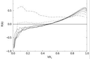
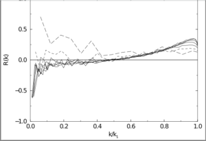
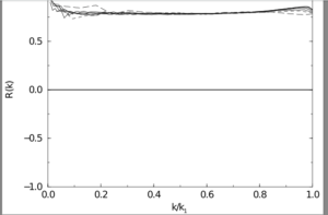
We carried out a numerical simulation of stationary, isotropic turbulence, with the velocity field in wavenumber defined on the interval $0\leq k \leq k_0$. Various cut-off wave numbers $k_1 \leq k_0$, $k_2 \leq k_1$, $k_3 \leq k_2$; and so on, were considered, so that a series of large-eddy simulations could be compared to the fully resolved simulation. I discussed in my post of 23 March 2023 how the complex velocity field in wavenumber (a.k.a the Fourier transform of the real-space velocity field) could be separated into amplitude and phase; and this was the method employed in [3], from which I have taken three figures. In all cases, we evaluated a correlation coefficient $R(k)$ and this is plotted against $k/k_$, where $k_1$ is the maximum resolved wavenumber in all cases.

In Figure A, we show the correlation $R(k)$ between the subgrid stresses and the eddy viscosity for seven cut-off wavenumbers in the range $16.5 \leq k_1 \leq 112.5$ with $k_0 = 128$. It can be seen that for most cases (shown by continuous lines) the correlation is not very good, varying from $0.25 – 0.5$ at the cut-off wavenumber to essentially being anti-correlated as $h/k_1 \rightarrow 0$. The exceptions are the curves for the lowest cut-off wavenumbers $k_1 =16.5$ (long dashes) and $k_1= 32.5$ (short dashes); and in particular the first of these. It should be noted that the first of these is the only one to yield a finite plateau region in the plot of the effective viscosity against wavenumber [3]. This latter property is an indication that it is only this lowest cut-off wavenumber which gives an adequate degree of scale separation compared to the maximum value.

FIG A

In Figure B, we show the phase correlations for the same cases, and the similarity to the results of Figure A are quite marked.

FIG B

On the other hand, the results for amplitude correlations in Figure C show a high level of correlation over the entire range of wavenumbers, with very little variation between the results for the various cut-off wavenumbers.

FIG C

In this case, isotropic turbulence, we are mainly interested in modelling the inertial transfer through wavenumber and for this purpose a model which represents the amplitudes is quite effective. However, given that all such formulations are based on average quantities it is not easy to see how the phases can be taken into account.

[1] W. David McComb. Homogeneous, Isotropic Turbulence: Phenomenology, Renormalization and Statistical Closures. Oxford University Press, 2014.
[2] O. J. McMillan and J. H. Ferziger. Direct testing of subgrid-scale models. AIAA Journal, 17:1340, 1979.
[3] W. D. McComb and A. J. Young. Explicit-Scales Projections of the Partitioned Nonlinear Term in Direct Numerical Simulation of the Navier-Stokes Equation. Presented at 2nd Monte Verita Colloquium on Fundamental Problematic Issues in Turbulence: available at arXiv:physics/9806029 v1, 1998.

Mode elimination: taking the phases into account: 4

In the previous post we came to the unsurprising conclusion that as a matter of rigorous mathematics, we cannot average out the high-wavenumber modes while leaving the low-wavenumber modes unaffected. However, turbulence is a matter of physics rather than pure mathematics and the initial conditions are not known with mathematical precision. Here the concept of deterministic chaos comes to our rescue. If we accept that the initial condition must have some uncertainty attached to it, then there is a possibility that such an average can be carried out approximately.

We can generalise the conditional average, given as equation (3) in the previous post, by extending it to some arbitrary well-behaved functional $H[u(k,t)]$. Here we are also using the simplified notation of the previous post; and in fact we shall simplify it even further, and write $u(k,t)\equiv u_k$. Then we can replace that equation by:\begin{equation}\langle H[u_k]\rangle_c = \langle H[u_k]\mid u^-_k \rangle,\end{equation} where, as before, the subscript `$c$’ on the left hand side denotes `conditional average’; and the notation on the right hand side indicates that the ensemble average is carried out while keeping the low-wavenumber part of the velocity field $ u^-_k$ constant. From the previous discussion, we know that this average amounts to a delta function, as both $u_k$ and $u^+_k$ are also held constant.

The way out of this impasse is the recognition that, in the real physical situation, $u^-_k$ cannot be held precisely to any exact value. There must be some uncertainty, however small, in the application of this constraint. Accordingly we introduce an uncertainty into our definition of a conditional average by writing it as: \begin{equation}\langle H[u_k]\rangle_c = \langle H[u_k]\mid u^-_k + \phi^-_k\rangle.\end{equation} Evidentally, $ u^-_k + \phi^-_k$ must be a solution of the Navier-Stokes equation, but the uncertainty $\phi^-_k$ is otherwise arbitrary and may be chosen to have convenient properties. In fact, McComb, Roberts and Watt [1] chose it to satisfy the conditions:\begin{equation} \langle u^-_k\rangle_c = u^-_k + \langle \phi^-_k \rangle_c,\end{equation} along with:\begin{equation} \langle u^-_k u^-_j\rangle_c = u^-_k + \langle \phi^-_k \phi^-_j \rangle_c,\end{equation} and \begin{equation} \langle u^-_ku^+_j\rangle_c = u^-_k \langle u^+_k \rangle_c.\end{equation} These relationships are then used in decomposing the NSE and implementing an RGl calculation. It should be noted that $ \langle u^+_k \rangle_c$ is not zero and an equation of motion must be derived for it.

The problem posed by the correction terms in $\phi^-_k$ depends on just how chaotic the turbulence is, but the calculations suggest that these terms can be neglected. In fact the calculation of the invariant energy flux yields a value of the Kolmogorov spectral constant of $\alpha = 1.62$ which is the generally accepted value. Further details can be found in the original paper [1] and in the appropriate sections of the book [2].

However, despite the above procedures, there are still phase effects that are not being taken into account, and this will be the subject of the next post.

[1] W. D. McComb, W. Roberts, and A. G. Watt. Conditional-averaging procedure for problems with mode-mode coupling. Phys. Rev. A, 45(6):3507- 3515, 1992.
[2] W. David McComb. Homogeneous, Isotropic Turbulence: Phenomenology, Renormalization and Statistical Closures. Oxford University Press, 2014.