Superstitions in turbulence theory 2: that intermittency destroys scale-invariance!

At the moment I am busy revising a paper (see [1] below) in order to meet the comments of the referees. As is so often the case, Referee 1 is supportive and Referee 2 is hostile. Naturally, Referee 2 writes at great length, so it is really a matter of rebuttal rather than our making changes. It seems clear that he is far from his comfort zone and his comments show that he has comprehensively misunderstood our paper. It also seems to me that he has not actually read certain key parts of the manuscript. For instance, he states: ‘The way how the authors use the word “scale-invariance” should be clarified’ (sic).

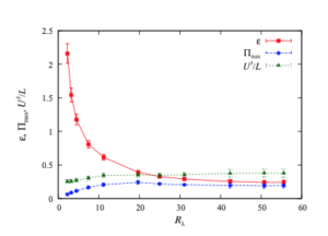
This is despite the fact that subsection 3.1 of the paper is titled ‘Scale-invariance of the inertial flux in the infinite Reynolds number limit’ and consists of only three paragraphs. It contains two equations, one of which states the criterion for an inertial range. This is followed by a sentence ending with “… where the fact that the criterion holds over a range of wavenumbers is usually referred to as scale-invariance.” Oh, and as regards ‘how the authors use the word’, we cite a number of references to show that others use the phrase, so we are not alone.

The next thing he says is: ‘We know from experimental evidence (intermittency) that scale invariance is broken in the inertial range.’ This is quite simply nonsense. In this context scale-invariance means that the inertial range is characterised by a constant flux over a range of wavenumbers, and this has been shown in many investigations. In fact there is no way in which intermittency, which is a single-realization characteristic, can affect mean quantities such as inertial flux or their properties such as scale-invariance. In a recent paper [2], we have shown that the ensemble average of intermittency vanishes. In the first figure below, we show the effect of using contours of isovorticity and the progressive effect of averaging over $N=1,\,2,\,5,\,10,\,25$ and $46$ realizations.

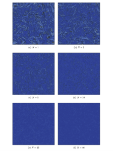
The effect of the averaging out with increasing number of realizations is evident. While the use of vorticity is more natural, the effect can perhaps be more clearly seen using the Q-criterion, as is done in the next figure.

 

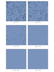
Both figures are taken from the same stationary DNS of the Navier-Stokes equations. Further details can be found in reference [2].

Over the past three decades there has been an increasing body of evidence to the effect that intermittency does not affect the Kolmogorov spectrum. Any deviations are in fact due to the Kolmogorov conditions not being quite met. Presumably it will take a long time for rational enquiry to defeat superstition in this topic!

[1] W. D. McComb and S. R. Yoffe. The infinite Reynolds number limit and the quasi-dissipative anomaly. arXiv:2012.05614v2[physics.flu-dyn], 2021.
[2] S. R. Yoffe and W. D. McComb. Does intermittency affect the inertial transfer rate in stationary isotropic turbulence? arXiv:2107.09112v1 [physics.flu-dyn], 2021.

Superstitions in turbulence theory 1: the infinite Re limit of the Navier-Stokes equation is the Euler equation!

I recently posted blogs about the Onsager conjecture [1]; the need to take limits properly (Onsager didn’t!); and the programme at MSRI Berkeley, which referred to the Euler equation as the infinite Reynolds number limit, in a series of posts from 5 – 19 August just past. A later notification about the MSRI programme no longer made that claim; and I speculated (conjectured?) that this might not be unconnected from the appearance of the paper [2] on the arXiv! Now the Isaac Newton Institute is having a new programme on mathematical aspects of turbulence over the first half of next year, and their theme dwells on how the mathematics underlying ‘the proof of the Onsager conjecture … can bring insights into the dissipative anomaly conjecture, a.k.a. Kolmogorov’s zeroth law of turbulence’.

The idea of a dissipation (or dissipative) anomaly goes back to Onsager’s conjecture [1] made in 1949 when turbulence studies were still in their infancy. Although the alternative expression (i.e Kolmogorov’s zeroth law) has also been used, I have no idea who formulated it; nor of the reasoning that lies behind it. While Kolmogorov may have formulated laws in statistics (I am indebted to Mr Google for this information!), his contributions to turbulence do not qualify for the description ‘physical laws’. However, an irony about the way in which Onsager came to his conclusion about a dissipative anomaly recently dawned on me, and the point of this post is to share that with you.

Onsager’s starting point was Taylor’s (1935) expression for the turbulent dissipation [3] thus: \begin{equation}\varepsilon = C_{\varepsilon}(R_L) U^3/L,\end{equation} where $\varepsilon$ is the dissipation rate, $U$ is the root mean square velocity, $L$ is the integral scale, and $C_{\varepsilon}$ is a coefficient which may depend on the Reynolds number $R_L$, which is formed from the integral scale and the rms velocity. In 1953, Batchelor [4] presented some results that suggested $C_{\varepsilon}$ tended to a constant with increasing Reynolds number.. Nevertheless, this expression was the subject of some debate over the years (although its equivalent for shear flows was widely used in both research and practical applications), until Sreenivasan’s survey papers on grid turbulence [5] in 1984 and on direct numerical simulations [6] in 1998 established the characteristic asymptotic shape of this curve. This work had a seminal effect on the subject and a general account of work in this area can be found in the book [7].

However, it was suggested by McComb et al in 2010 [8] that the Taylor’s expression for the dissipation (1) is actually a surrogate for the peak inertial flux $\Pi_{max}$. See the figure below, which is taken from that paper. It shows from DNS that the group $U^3/L$ behaves like $\Pi_{max}$ for all Reynolds numbers, whereas the behaviour of the dissipation is quite different at low Reynolds numbers.

It was further shown [9], using the Karman-Howarth equation and expanding non-dimensional structure functions in inverse powers of the Reynolds number, that this was the case, with the asymptotic behaviour $C_{\varepsilon} \rightarrow C_{\varepsilon,\infty}$ as $R_L \rightarrow \infty$ corresponding to the onset of the Kolmogorov $`4/5’$ law.

In other words, when Onsager deduced from Taylor’s expression that the dissipation did not depend on the viscosity, he was actually deducing that the peak inertial flux did not depend on the viscosity. And indeed it doesn’t!

[1] L. Onsager. Statistical Hydrodynamics. Nuovo Cim. Suppl., 6:279, 1949.
[2] W. D. McComb and S. R. Yoffe. The infinite Reynolds number limit and the quasi-dissipative anomaly. arXiv:2012.05614v2[physics.flu-dyn], 2021. 28.
(N.B. This paper is presently under revision and will be posted again, possibly with a change of title.)
[3] G. I. Taylor. Statistical theory of turbulence. Proc. R. Soc., London, Ser. A, 151:421, 1935.
[4] G. K. Batchelor. The theory of homogeneous turbulence. Cambridge University Press, Cambridge, 1st edition, 1953.
[5] K. R. Sreenivasan. On the scaling of the turbulence dissipation rate. Phys. Fluids, 27:1048, 1984.
[6] K. R. Sreenivasan. An update on the energy dissipation rate in isotropic turbulence. Phys. Fluids, 10:528, 1998.
[7] W. David McComb. Homogeneous, Isotropic Turbulence: Phenomenology, Renormalization and Statistical Closures. Oxford University Press, 2014.
[8] W. David McComb, Arjun Berera, Matthew Salewski, and Sam R. Yoffe. Taylor’s (1935) dissipation surrogate reinterpreted. Phys. Fluids, 22:61704, 2010.
[9] W. D. McComb, A. Berera, S. R. Yoffe, and M. F. Linkmann. Energy transfer and dissipation in forced isotropic turbulence. Phys. Rev. E, 91:043013, 2015.

Peer review: the role of the referee.
In earlier years I used to get the occasional phone call from George Batchelor, at that time the editor of Journal of Fluid Mechanics, asking for suggestions of new referees on the statistical theory of turbulence. To avoid confusion I should point out that by this I mean the theoretical physics approach to the statistical closure problem, pioneered by Bob Kraichnan and Sam Edwards, and carried on by myself and others. For anyone interested, a review of this subject can be found in reference [1] below.

I didn’t find this easy, as there were then (as now) very few people working on this topic. My suggestion that Sam Edwards, although no longer active in this area, could certainly referee papers, was met with little enthusiasm. He was seen as ‘too kind’ or even as ‘soft-hearted’! I wasn’t surprised by this, as Sam had explained his position on refereeing to me and it amounted to: ‘Unless it is arrant nonsense, it should be published.’ In contrast, the refereeing process of the JFM was notoriously tough and this has been generally true in turbulence research, and remains so to this day. Indeed this is the general perception in the subject, and to quote Sam again, he once referred to ‘the cut-throat nature of refereeing in turbulence’. I suspect it was this perception which put him off continuing in the subject.

I find myself somewhere between the extremes, perhaps because this is a matter of culture and I have been both engineer and physicist. However, while I respect the professionalism of the engineering approach, at the same time I think it can be taken too far. A typical experience for me (and I believe also for many others) is that a technical discussion can be carried on between the authors and individual referees which is never seen by others in the field. In my view these discussions should be published as an appendix to the paper (assuming of course that the paper is actually accepted for publication). I also think that where the authors have a track record there should be a presumption that the paper should be published. In other words, the onus should be on the referee to come up with definite and reasoned objections, as opposed to the vague prejudiced waffle which is so often the case!

Another problem that arises often in the turbulence community, is the desire of some referees to rewrite the paper. Or rather to force the author(s) to rewrite the paper to the referee’s prescription. It is of course legitimate to point out aspects which are less clear than they might be, but it verges on arrogance to tell the author how to do it. Also, with electronic publication now universal the idea of saving paper/printing costs is no longer so relevant. Papers can easily be as long as they need to be.

I have been on the receiving end of this behaviour on occasion, but nothing compared to something I was told recently; where a leading member of the community was forced to modify his paper four times despite his own judgement that the changes were unnecessary and his making protests to that effect to the editor. Someone else I know, summed it up as ‘lazy editors and biased referees’. He had come from particle physics, where his papers had generally been published ‘as submitted’, to fluid mechanics (in the context of climatology) where there was invariably a battle over changes being required by the referee. Of course I trust that it is clear that I am not referring to the minor changes that we should all be happy to make, but to major structural changes which may in the end be no more than one person’s opinion against another’s. For these two individuals it was the failure by the editors to intervene that caused the problems.

So, it really comes down to the editor in the end. It is their job to protect their referees from unfair attack, on the one hand; and to protect their authors from unfair refereeing, on the other. As I have pointed out elsewhere, in practice what breaks this symmetry is that it is more difficult for the editor to get referees than it is to get prospective authors; who, after all, are queuing up to apply!

[1] W. D. McComb and S. R. Yoffe. A formal derivation of the local energy transfer (LET) theory of homogeneous turbulence. J. Phys. A: Math. Theor., 50:375501, 2017.

Peer review: The role of the author.
I have previously posted on the role of the editor (see my blog on 09/07/2020) and had intended to go on to discuss the role of the referee. However, before doing that it occurred to me that it might be helpful to first discuss the role of the author. Of course probably every journal lays down rules for author and referee alike: but who pays any attention to these? (Just joking! Although, life is short and if you are having to try more than one journal, then the fact that these detailed rules vary from one journal to another can add to the labour involved.) But what I have in mind are the unwritten rules. These are generally taken for granted and perhaps should be spelled out occasionally in order to ensure that everyone is on the same wavelength.

One basic rule for authors is that they should provide some basic introduction to the problem, discuss previous work and show how their own new work advances the situation. This is very much in our own interest, as it is a key part of demonstrating to our co-workers that our paper is worth reading. However, as I found out at the beginning of my career, this is can be a fraught process. For instance, writing the introduction to a paper on the statistical theory of turbulence was perfectly straightforward, but in the case of an attempted theory of drag reduction by additives this turned out to be quite another matter.

My attention was drawn to this problem when I was in the Theoretical Physics Division at Harwell. At first this involved polymer molecules; but, when I looked into it further, I found out that there was a parallel activity based on the use of macroscopic fibres such as wood-pulp or rayon. This latter activity generally seemed to have originated within the relevant industry, and was often carried on without reference to the better known use of polymer additives.

I found the fibre problem more attractive, because it seemed easier to think about a macroscopic fibre as a linear object which could only have two-dimensional interactions with a three-dimensional eddy of comparable size. If one added in the possibility of elastic deformation of the fibre by the fluid, then one could think in terms of a non-Newtonian relationship between stress and rate of strain for the composite fluid which could act as a model for the fibre suspension. On the assumption that the fibres would tend to be aligned (on average) with the mean flow, physical reasoning led to an expression for a nonlinear correction to the usual Newtonian viscosity, which could be further decomposed into the difference between two-dimensional and three-dimensional inertial transfer terms, both of which represented reversals of the usual energy cascade. This theory offered a qualitative explanation of the changes in turbulent intensities which had been observed in fibre suspensions and was published as a letter in Nature [1].

So far so good! The problems arose when I extended this work and submitted it to JFM. All three referees were unanimous in rejecting the paper. Part of the trouble seemed to be that the work was carried out in spectral space. An account of this can be found in my blog of 20/02/2020, including the infamous description of my analysis as ‘the usual wavenumber murder’! But, as was kindly pointed out to me by George Batchelor, the problem was that I was ‘treading on the toes’ of those who worked in this field (i.e. microrheology). This editorial advice was helpful; because, from my background in physics, I knew very little about fluid mechanics and was happily unaware that the subject of microrheology even existed.

Of course, in the spirit of ‘poacher turned gamekeeper’ I ultimately became very keen on making sure that any paper of mine had a proper literature survey. I owe this mainly to my PhD students, who have always been very assiduous in tracking down references, and who have set me a good example in this respect!
Nowadays, in view of the great increase in publications, I tend to take a more tolerant attitude to others who fail to cite relevant papers. But I’m not sure that this is really justified. After all, although we have had a positive explosion of publications in fluid mechanics, most of this is in practical applications. The amount of truly fundamental work is still quite small. And we do have the power of Google to help us find anything that is relevant to what we are currently publishing. I must say that I am rather sceptical about papers that purport to present applications of theoretical physics to turbulence yet do not mention the name ‘Kraichnan’. I suspect them of being fake theories. This is something that I may expand on sometime.

For those who are interested, a further account of developments in the study of drag reduction may be found in my book cited as [2] below.

[1] W. D. McComb. The turbulent dynamics of an elastic fibre suspension: a mechanism for drag reduction. Nature Physical Science, 241(110):117-118, 1973.
[2] W. D. McComb. The Physics of Fluid Turbulence. Oxford University Press, 1990.

The exactness of mathematics and the inexactness of physics.

This post was prompted by something that came up in a previous one (i.e. see my blog on 12 August 2021), where I commented on the fact that an anonymous referee did not know what to make of an asymptotic curve. The obvious conclusion from this curve, for a physicist, was that the system had evolved! There was no point in worrying about the precise value of the Reynolds number. That is a matter of agreeing a criterion if one needs to fix a specific value. But evidently the ratio shown was constant within the resolution limits of the measurements of the system; and this is the key point. Everything in physics comes down to experimental error: the only meaningful comparison possible (i.e. theory with experiment or one experiment with another) is subject to experimental error which is inherent. Strictly one should always quote the error, because it is never zero.

In everyday life, there are of course many practical expedients. For instance, radioactivity takes in principle an infinite amount of time to decay completely, so in practice radioisotopes are characterised by their half-life. So the manufacturers of smoke alarms can tell you when to replace your alarm, as they know the half-life of the radioactive source used in it. In acoustics or diffusion processes or electromagnetism, exponential decays are commonplace, and it is usual to introduce a relaxation time or length, corresponding to when/where the quantity of interest has fallen to $1/e$ of its initial value.

In fluid mechanics, the concept of a viscous boundary layer on a solid surface is of great utility in reconciling the practical consequences of a flow (such as friction drag) with the elegance and solubility of theoretical hydromechanics. The boundary layer builds up in thickness in the stream-wise direction as vorticity created at the solid surface diffuses outwards. But how do we define that thickness? A reasonable criterion is to choose the point where the velocity in the boundary layer is approximately equal to the free-stream velocity. From my dim memory of teaching this subject several decades ago, a criterion of $u_1(x_2) = U_1$, where $U_1$ is the constant free-stream velocity, was adequate for pedagogic purposes.

An interesting partial exception arises in solid state physics, when dealing with crystal lattices. The establishment of the lattice parameters is of course subject to the usual caveats about experimental error, but for statistical physics lattices are countable systems. So if one is carrying out renormalization group calculations (e.g see [1]) then one is coarse-graining the description by replacing the unit cell, of side length $a$, by some larger (renormalized) unit cell. In wavenumber (momentum) space, this means we start from a maximum wavenumber $k_{max}=2\pi/a$ and average out a band of wavenumber modes $k_1 \leq k \leq k_0$, where $k_0=k_{max}$. You can see where the countable aspect comes in, and of course the initial wavenumber is precisely defined (although of course its precise value is subject to the error made in determining the lattice constant).

When extending these ideas to turbulence, the problem of defining the maximum wavenumber is not solved so easily. Originally people (myself included) used the Kolmogorov dissipation wavenumber, but this is not necessarily the maximum excited wavenumber in turbulence. In 1985 I introduced a criterion which was rather like a boundary-layer thickness, adapting the definition of the dissipation rate, thus: \[\varepsilon = \int^{\infty}_0 \, 2\nu_0 k^2 E(k) dk \simeq \int^{k_{max}}_0 \, 2\nu_0 k^2 E(k) dk,\] where $\nu_0$ is the molecular viscosity and $E(k)$ is the energy spectrum [2]. When I first started using this, physicists found it odd, because they were used to the more precise lattice case. I should mention for completeness that it is also necessary to use a non-trivial conditional average [3].

Recently there has been growing interest in these matters by those who study the philosophy of maths and science. For instance, van Wierst [4] notes that in the theory of critical phenomena, phase transitions require an infinite system, whereas in real life they take place in finite (and sometimes quite small!) systems. She argues that this paradox can be resolved by the introduction of ‘constructive mathematics’, but my view is that it can be adequately resolved by the concept of scale-invariance. Which brings us back to the infinite Reynolds number limit for turbulence. But, for the moment, I have said enough on that topic in previous posts, and will not expand on it here.

[1] W. D. McComb. Renormalization Methods: A Guide for Beginners. Oxford University Press, 2004.
[2] W. D. McComb. Application of Renormalization Group methods to the subgrid modelling problem. In U. Schumann and R. Friedrich, editors, Direct and Large Eddy Simulation of Turbulence, pages 67-81. Vieweg, 1986.
[3] W. D. McComb and A. G. Watt. Conditional averaging procedure for the elimination of the small-scale modes from incompressible uid turbulence at high Reynolds numbers. Phys. Rev. Lett., 65(26):3281-3284, 1990.
[4] Pauline van Wierst. The paradox of phase transitions in the light of constructive mathematics. Synthese, 196:1863, 2019.