That’s the giddy limit!

That’s the giddy limit!
Staycation post No 2. I will be out of the virtual office until 30 August.

The expression above was still in use when I was young, and vestiges of its use linger on even today. It referred, often jocularly, to any behaviour which was deemed unacceptable. Why giddy? I’m afraid that the reference books are silent on that. However, I have encountered examples of mathematical limits which seemed to qualify for the adjective.

Shortly before I retired, I found myself teaching a mathematics course to third-year physics students. The purpose of this course was to try to bring our students up to speed in maths, after the mathematics lecturers had done their best in the previous two years. I suppose that it had a remedial aspect, and at that time the talk was all of the ‘math problem’. One example of a ‘giddy’ limit, which sticks in my mind, arose when I was marking class exam papers. The question asked the students to sketch the function $sinc \,\nu = \sin \nu / \nu$. This required them to work out its value at $\nu =0$, where of course direct substitution results in an indeterminate form. I need hardly say that they had to use either a Taylor series expansion of $sin$ or make use of l’Hopital’s rule to reveal the correct limiting value which is unity. Or of course they could just sketch it and infer the limiting behaviour by eye.

One person did this beautifully, with all the zeros in the right places and the central peak heading up to the value one on both sides. It was as the $y$-axis was approached that giddiness seemed to set in, and the sketched curve then shot down to zero on both sides. The student then proudly declared it to be an indeterminate form. One, which just happened to be zero! This sudden abandonment of all reason was quite baffling and I never understood the reason for it.

However, I recently saw comments by an anonymous referee which seemed to come into a similar category. These were directed at Figure 2 in reference [1] which was intended to demonstrate that the physical infinite Reynolds number limit was determined by the onset of scale-invariance. We show this below. Scale-invariance in this context is defined to be when the maximum rate of inertial transfer $\varepsilon_T$ becomes equal to the viscous dissipation $\varepsilon$. As we were originally studying the dependence of dimensionless dissipation of Taylor-Reynolds number, we actually plot the ratio $ \varepsilon / \varepsilon_T $, which reduces towards unity, and this indicates the onset of scale-invariance.

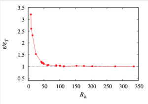
The referee looked at the figure and asked: how is the onset of scale-invariance defined? Is the onset placed at $R_{\lambda}=50,\,100\,150$?

This seems to me to verge on the childish. Does he have no familiarity with the intersection between a mathematically asymptotic result and a real physical system? Has he never met viscous boundary layers, exponential decay of sound or other radiation? The answer in all these cases is set by the resolution of the physical measuring system. Once changes are too small to be measurable, then the asymptote has been reached. The curve that we show in the figure, would go on at a constant level no matter how much one increased the Reynolds number.

The lesson to be drawn from this is that there are no further qualitative changes in the system as you increase the Reynolds number, and this is how real fluids behave. In the next blog we will consider the motivation for the research reported in [1].

[1] W. D. McComb and S. R. Yoffe. The infinite Reynolds number limit and the quasi-dissipative anomaly. arXiv:2012.05614v2[physics.flu-dyn], 2021.