The Kolmogorov (1962) theory: a critical review Part 2
The Kolmogorov (1962) theory: a critical review Part 2
Following on to last week’s post, I would like to make a point that, so far as I know, has not previously been made in the literature of the subject. This is, that the energy spectrum is (in the sense of thermodynamics) an intensive quantity. Therefore it should not depend on the system size. This is, as opposed to the total kinetic energy (say) which does depend on the size of the system and is therefore extensive.
What applies to the energy spectrum also applies to the second-order structure function. If we now consider equation (1) from the previous blog, which is \begin{equation}S_2(r)=C(\mathbf{x},t) \varepsilon^{2/3}r^{2/3}(L/r)^{-\mu}, \label{62S2}\end{equation}then for isotropic, stationary turbulence, it may be written as: \begin{equation}S_2(r)=C \varepsilon^{2/3}r^{2/3} (L/r)^{-\mu}. \end{equation} Note that $C$ is constant, as it can no longer depend on the macrostructure.
Of course this still contains the factor $L^{-\mu}$. Now, $L$ is only specified as the external scale in K62, but it is necessarily related to the size of the system. Accordingly taking the limit of infinite system size, is related to taking the limit of infinite values of $L$, which is needed in order to have $k=0$ and to be able to carry out Fourier transforms. If we do this, we have three possible outcomes. If $\mu$ is negative, then $S_2 \rightarrow \infty$, as $L \rightarrow \infty$, whereas if $\mu$ is positive, then $S_2$ vanishes in the limit of infinite system size. Hence, in either case, the result is unphysical, both by the standards of continuum mechanics and by those of statistical physics.
However, if $\mu = 0$ then there is no problem. The structure function (and spectrum) exist in the limit of infinite system size. Could this be an argument for K41?
Lastly, we should mention that McComb and May [1] have used a plausible method to estimate values of $L$ and, taking a representative value of $\mu=0.1$, have shown that the inclusion of this factor as in K62 destroys the well-known collapse of spectral data that can be achieved using K41 variables.
We began with the well-known graph in which one-dimensional projections of the energy spectrum for a range of Reynolds numbers are normalized on Kolmogorov variables and plotted against $k’=k/k_d$: see, for example, Figure 2.4 of the book [2], which is shown immediately below this text.
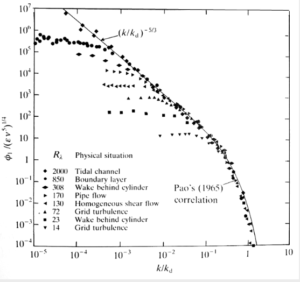
In this work, we referred to $L$ as $L_{ext}$ and we estimated it as follows. From the above graph, we see that the universal behaviour always occurs in the limit $R_\lambda \rightarrow \infty$ with all spectra collapsing to a single curve at $k’= k/k_d =1$. As the Reynolds number increases, each graph flattens off as $k$ decreases and ultimately forms a plateau at low wavenumbers. We argued that one can use the point where this departure takes place $k’_{ext}$ (say) to estimate the external length scale, thus; \[L’_{ext} = 2\pi/k’_{ext}.\]
In order to make a comparison, we chose the results for a tidal channel at $R_{\lambda}=2000$ and for grid turbulence at $R_{\lambda}=72$. We show these two spectra, as selected from Fig. 1, on Figure 2 below.
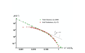
Note that we plot the scaled one-dimensional spectrum $\psi(k’)=\phi(k’)/(\varepsilon \nu^5)^{1/4}$.
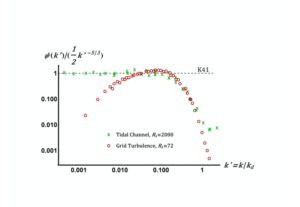
In the next figure, we plot these two spectra in compensated form, where we have taken the one-dimensional spectral constant to be $\alpha_{1}=1/2$, on the basis of Figure 2. In this form the $-5/3$ power law appear as a horizontal line at unity. We will return to this aspect later.
In order to assess the effect of including the K62 correction, we estimated to be $L’_{ext}\sim 50$ for the grid turbulence and as $L’_{ext}\sim 2000$ for the tidal channel. In fact the spectra from the tidal channel do not actually peel off from the $-5/3$ line at low $k$ so our estimate is actually a lower bound for this case. This favours K62 in the comparison. We took the value $\mu = 0.1$, as obtained by high-resolution numerical simulation and the result of including the K62 correction is shown in Figure 4.
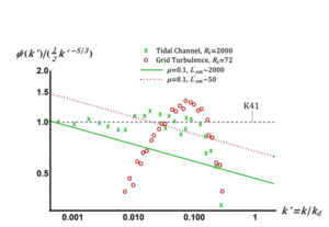
It can be seen that including the K62 corrections destroys the collapse of the spectra which, apart from showing a slope of $\mu = -0.1$ in both cases, are now separated and in a constant ratio of $0.69$. Evidently the universal collapse of spectra in Figure 1 would not be observed if the K62 corrections were in fact correct!
My final point is that one of the unfavourable referees for this paper had a major concern with the fact that the results for grid turbulence did not really show much $-5/3$ behaviour. This is to miss the point. The K41 scaling shows a universal form in the dissipation range, as well as in the inertial range. The inclusion of the K62 correction destroys this, when implemented with plausible estimates for the two parameters.
[1] W. D. McComb and M. Q. May. The effect of Kolmogorov (1962) scaling on the universality of turbulence energy spectra. arXiv:1812.09174[physics.flu-dyn], 2018.
[2] W. D. McComb. The Physics of Fluid Turbulence. Oxford University Press, 1990.