The modified Lin equation.

The modified Lin equation.

In my post of 27 February I discussed the importance of being aware of the full form of the Lin equation as this reveals the existence of a cascade in wavenumber space. In this post I want to take this a bit further, using my resolution of the scale-invariance paradox [1].

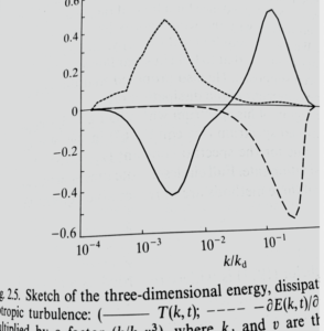
For me this topic first arose during a meeting in 1991 at MSRI, Berkeley. When I had finished my talk, Bob Kraichnan came up to me with a copy of my recently published book and pointed out Figure 2.5, which was a plot of the terms in the Lin equation for freely decaying turbulence. He commented on the fact that the transfer spectrum $T(k)$ was shown as zero for an extended range of values of $k$. He commented that people used to think that was the case, because it would be expected from the scale-invariance of the flux, but that in practice it was never observed. There was always a single zero-crossing. I was able to reassure him that figure was based on a computation of the LET theory; that there had been an error which had now been rectified; and that the revised figure would show a single zero-crossing and would appear in the paperback edition of the book to be published later that year.

However, I was left with a nagging feeling that there was an unresolved problem with this result. The first measurements of $T(k)$ had been published by Uberoi [2] in 1963, and this author had said that the single zero-crossing was probably due to the low Reynolds number and indicated that he would expect $T(k)=0$ over an extended range of $k$ to develop with increasing Reynolds number. Although this does not seem to have been a matter of widespread concern, over the 1970s/80s/90s various ad hoc methods were used to cope with this behaviour in numerical calculations: for some references to this work, see [1]. As a matter of interest, I include both versions of Figure 2.5 below.

 

 

 

 

 

 

 

 

 

 

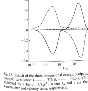
The Lin equation (see reference [3]) takes the form: \begin{equation} \left( \frac{d}{dt} + 2 \nu k^2 \right) E(k,t) = T(k,t)\label{enbalt}\end{equation} where $E(k,t)$ is the energy spectrum, $T(k,t)$ is the energy transfer spectrum and $\nu$ is the kinematic viscosity. Now let us integrate each term of (\ref{enbalt}) with respect to wavenumber, from zero up to some arbitrarily chosen wavenumber $\kappa$: \begin{equation} \frac{d}{dt}\int_{0}^{\kappa} dk\, E(k,t) = \int^{\kappa}_{0} dk\, T(k,t)-2 \nu\int_{0}^{\kappa} dk\, k^2 E(k,t). \label{fluxbalt1} \end{equation} The energy transfer spectrum may be written as \begin{equation} T(k,t) = \int^{\infty}_{0} dj\, S(k,j;t), \label{ts}\end{equation} where, as is well known, $S(k,j;t)$ can be expressed in terms of the triple moment. Its antisymmetry under interchange of $k$ and $j$ guarantees energy conservation in the form: \begin{equation}\int^{\infty}_{0} dk\, T(k,t) =0. \label{encon} \end{equation}

With some use of the antisymmetry of $S$, along with equation (\ref{encon}), equation (\ref{fluxbalt1}) may be written as \begin{equation}\frac{d}{dt}\int_{0}^{\kappa} dk\, E(k,t) = – \int^{\infty}_{\kappa} dk\,\int^{\kappa}_{0} dj\, S(k,j;t)-2 \nu\int_{0}^{\kappa} dk\, k^2 E(k,t).\label{fluxbalt2}\end{equation} the integral of the transfer term is readily interpreted as the net flux of energy from wavenumbers less than $\kappa$ to those greater than $\kappa$, at any time $t$.

It is convenient to introduce a specific symbol $\Pi$ for this energy flux, thus: \begin{equation}\Pi (\kappa,t) = \int^{\infty}_{\kappa} dk\, T(k,t) =-\int^{\kappa}_{0} dk\,T(k,t),\label{tp}\end{equation} where the second equality follows from (\ref{encon}).

The key to resolving the paradox is to introduce transfer spectra which have been filtered with respect to $k$ and which have had their integration over $j$ partitioned at the filter cut-off, i.e. $j=k_c$ [1],[4]. Beginning with the Heaviside unit step function, defined by:
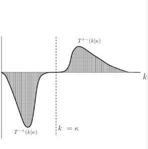
\begin{eqnarray} H(x) & = & 1 \qquad \mbox{for} \qquad x > 0; \\& = & 0 \qquad \mbox {for} \qquad x < 0.\end{eqnarray} we may define low-pass and high-pass filter functions, thus: \begin{equation}\theta^{-}(x) = 1 – H(x),\end{equation} and \begin{equation} \theta^{+}(x) = H(x). \end{equation} We may then decompose the transfer spectrum, as given by (\ref{ts}), into four constituent parts, \begin{equation}T^{–}(k|k_{c}) = \theta^{-}(k-k_{c})\int^{k_{c}}_{0}dj\, S(k,j); \label{tmm}\end{equation} \begin{equation} T^{-+}(k|k_{c}) = \theta^{-}(k-k_{c})\int^{\infty}_{k_{c}}dj\, S(k,j); \label{tmp}\end{equation} \begin{equation} T^{+-}(k|k_{c}) = \theta^{+}(k-k_{c})\int^{k_{c}}_{0}dj\, S(k,j); \label{tpm} \end{equation} and \begin{equation}T^{++}(k|k_{c}) = \theta^{+}(k-k_{c})\int^{\infty}_{k_{c}}dj\, S(k,j),\label{tpp} \end{equation} such that the overall requirement of energy conservation is satisfied: \begin{equation} \int^{\infty}_{0}dk\left[T^{–}(k|k_{c}) + T^{-+}(k|k_{c}) + T^{+-}(k|k_{c}) + T^{++}(k|k_{c})\right] = 0. \end{equation}It is readily verified that the individual filtered/partitioned transfer spectra have the following properties: \begin{equation} \int^{k_{c}}_{0}dk\, T^{–}(k|k_{c}) = 0; \label{mm} \end{equation} \begin{equation} \int^{k_{c}}_{0}dk\, T^{-+}(k|k_{c}) = -\Pi(k_{c});\label{mp} \end{equation} \begin{equation}\int^{\infty}_{k_{c}}dk\, T^{+-}(k|k_{c}) = \Pi(k_{c}); \label{pm} \end{equation} and \begin{equation} \int^{\infty}_{k_{c}}dk\, T^{++}(k|k_{c}) = 0. \label{pp} \end{equation} Equation (\ref{fluxbalt1}) may be rewritten in terms of the filtered/partitioned transfer spectrum as: \begin{equation} \frac{d}{dt}\int^{k_{c}}_{0}dk\, E(k,t) = -\int^{\infty}_{k_{c}}dk\, T^{+-}(k|k_{c}) -2\nu_{0}\int^{k_{c}}_{0}dk\, k^{2}E(k,t). \label{fluxbaltmod} \end{equation} We note from equation (\ref{mm}) that $T^{–}(k|k_c)$ is conservative on the interval $[0,k_c]$, and hence does not appear in (\ref{fluxbaltmod}), while $T^{-+}(k|k_{c})$ has been replaced by $-T^{+-}(k|k_{c})$, using (\ref{mp}) and (\ref{pm}). Those working with DNS or analytical theory, can avoid the paradox by changing their definition of energy fluxes, from those given by (\ref{tp}), to the forms: \begin{equation} \Pi (\kappa,t) = \int^{\infty}_{\kappa} dk\, T^{+-}(k|\kappa,t) =-\int^{\kappa}_{0} dk\, T^{-+}(k|\kappa,t),\label{tpmod} \end{equation} where $T^{+-}(k|\kappa,t)$ is defined by (\ref{tpm}) and $T^{-+}(k|\kappa,t)$ by (\ref{tmp}). This is equivalent to (\ref{tp}); but, unlike it, avoids the paradox.

This behaviour is illustrated in the figure below, where we should note that $T^{-+}(k|\kappa)$ is defined below the cut-off wavenumber $\kappa = k_{c}$, and $-T^{+-}(k|\kappa)$ is defined above it.

 

 

This raises the question of how exactly the Lin equation should be written, in order to emphasise these properties. That will be the subject of a paper which is now in preparation [5]. It is worth making the point that the filtered-partitioned forms of the transfer spectrum have only been studied in the context of the subgrid modelling problem [4]. Given the much more powerful computers now available, it would undoubtedly be rewarding to study the role of these terms in the energy balance for a range of Reynolds numbers. I very much hope that someone will do this.

Acknowledgement: the above figure was suggested by John Morgan, who also prepared it.

[1] David McComb. Scale-invariance in three-dimensional turbulence: a paradox and its resolution. J. Phys. A: Math. Theor., 41:75501, 2008.
[2] M. S. Uberoi. Energy transfer in isotropic turbulence. Phys. Fluids, 6:1048, 1963.
[3] W. David McComb. Homogeneous, Isotropic Turbulence: Phenomenology, Renormalization and Statistical Closures. Oxford University Press, 2014.
[4] W. D. McComb and A. J. Young. Explicit-Scales Projections of the Partitioned Nonlinear Term in Direct Numerical Simulation of the Navier-Stokes Equation. In Proc. 2nd Monte Verita Colloquium on Fundamental Problematic Issues in Turbulence: available at arXiv:physics/9806029 v1, 1998.
[5] W. D. McComb. A modified Lin equation for the energy balance in isotropic turbulence. arXiv:2007.13622v1 [physics.flu-dyn] 27 Jul 2020