Turbulence as a quantum field theory: 2
Turbulence as a quantum field theory: 2
In the previous post, we specified the problem of stationary, isotropic turbulence, and discussed the nature of turbulence phenomenology, insofar as it is relevant to taking our first steps in a field-theoretic approach. Now we will extend that specification in order to allow us to concentrate on renormalization group or RG.
RG originated in quantum field theory in the 1950s, but is best known for its successes in critical phenomena in the 1970s, along with the creation of the new subject of statistical field theory. Essentially it began as a method of exploiting scale invariance, and ended up as a method of detecting it, and also establishing the conditions under which it would hold. It is most easily understood in the theory of ferromagnetism, where we can envisage a model consisting of lots of little atomic magnets on a lattice. These atomic magnets (or lattice spins) interact with each other and, if we call the interaction energy for any pair $J$, this energy appears in the partition function as $J/k_B T$, where $k_B$ is the Boltzmann constant, and $T$ is the absolute temperature. This quantity is the coupling constant.
Now RG consists of coarse-graining our microscopic description, and then re-scaling it, to see it we can get back to where we started. If so, that would be a fixed point. In practice, we might expect to carry out this transformation a number of times, in order to reach such a fixed point. So in effect we are progressively reducing the number of degrees of freedom. This involves some sort of partial average at each step, in contrast to a full ensemble average, which gets you down from lots of degrees of freedom to just a few numbers being needed to describe a system.
Actually, merely by waving our hands about, we can deduce something about the fixed points of our lattice model of a ferromagnet. If we consider very high temperatures, then the coupling strength will be reduced to zero. The lattice spins will have a Gaussian probability distribution. We can envisage that this will be a fixed point, as no amount of coarse-graining will change it from a purely random distribution. At the other extreme, as the temperature tends to zero, the coupling tends to infinity and there can be no random behaviour: the spins will all line up. Once again, perfect order cannot be changed by coarse graining, and this also is a fixed point. What happens in between these extremes is interesting. As the temperature is reduced from some very large value, clumps of aligned spins will occur as fluctuations. The size of these fluctuations is characterised by the correlation length. As the temperature approaches some critical value $T_c$ from above, the correlation length will tend to infinity. When this occurs, it is no longer possible to coarse-grain away the ordering, as it exists on all scales. This fixed point is the critical point of the lattice.
So, RG applied to the model identifies the high- and low-temperature fixed points, which are trivial; and the critical fixed point which corresponds to the onset of ferromagnetism. This is known as real space RG and I have given a fuller account (with pictures!) elsewhere [1]. For completeness, I should mention that the momentum-space analytical treatment involves Gaussian perturbation theory in order to evaluate parameters associated with the critical point. Also, the temperature in this context is known as a control parameter.
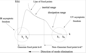
In turbulence, the degrees of freedom are the independently excited Fourier modes. The coupling parameter for each mode can be identified with Batchelor’s Reynolds number (see my earlier post on 23/04/20) which takes the form $R(k)=[E(k)]^{1/2}/\nu k^{1/2}$. Using the schematic energy spectrum, as given in the preceding post, we can identify the trivial fixed points where the coupling falls to zero. This is because the spectrum is known to go to zero at least as $k^4$ as $k\rightarrow 0$ and to zero exponentially as $k\rightarrow \infty$. By analogy with quantum field theory, we refer to these points as being asymptotically free in the infra-red and the ultra-violet, respectively. In order to compare with magnetism, we can argue that the $k=0$ fixed point is analogous with the high-temperature, where the low-$k$ motion is random (Gaussian) due to the stirring, whereas at large $k$, the motion is damped by viscosity and is analogous to the low-temperature fixed point. In the figure we identify another possible, but non-trivial, fixed point where the inertial range is represented by the Kolmogorov $k^{-5/3}$ spectrum. A power law, being scale-free, is likely to be associated with a fixed point of the RG transformations.
In order to carry out calculations, we seek to eliminate modes progressively in bands, first $k_1\leq k\leq k_0$, then $k_2 \leq k \leq k_1$, and so on. At the first stage, the effect of the missing modes results in an increase to the viscosity $\nu_0 \rightarrow \nu_1 = \nu_0 + \delta \nu_0$. We then rescale on the increased viscosity, and repeat the process. Note that we rename the molecular viscosity $\nu = \nu_0$ for this purpose. Also note that it can be a little counter-intuitive associating zero with the maximum value of $k$, but we want an increasing index as we reduce $k$, leading on to a recurrence relationship which may reach a fixed point.
In the theory of magnetism, the lattice spacing $a$ is used to define the maximum wavenumber, thus $k_{max} = 2\pi/a$. In turbulence, sometimes the Kolmogorov wavenumber is used for the maximum, but this is likely to be incorrect by at least an order of magnitude. A better definition has been given [2] in terms of the dissipation integral, thus: $\varepsilon = \int_0^\infty 2\nu_0 k^2 E(k) dk \simeq \int_0^{k_{max}}2\nu_0 k^2 E(k) dk$.
I shall highlight two calculations here. Forster et al [3] carried out an RG calculation by restricting the wavenumbers considered to a region near the origin. This was very much a Gaussian perturbation theory of the type used in the study of critical phenomena. They did not refer to this as turbulence, and instead considered it as the large scale asymptotic behaviour of randomly stirred fluid motion.
Later, McComb and Watt [4], introduced a form of conditional average which allowed the RG transformation to be formulated as an approximation, valid even at large wavenumbers. They were able to find a non-trivial fixed point which corresponded to the onset of the inertial (power-law) range and gave a good value of the Kolmogorov spectral constant. This work has been carried on and refined but is very largely ignored. In contrast, Forster et al seem to have established a new paradigm of Gaussian fluid motion which permits the application of much field theoretic RG which relies on the simplifications of the paradigm. There is, however, one difference. Nowadays people publishing in this field describe it as turbulence! The most up-to-date treatment of the conditional averaging method will be found in [5].
[1] W. D. McComb. Renormalization Methods. Oxford University Press, 2004.
[2] W. D. McComb. Application of Renormalization Group methods to the subgrid modelling problem. In U. Schumann and R. Friedrich, editors, Direct and Large Eddy Simulation of Turbulence, pages 67, 81. Vieweg, 1986.
[3] D. Forster, D. R. Nelson, and M. J. Stephen. Long-time tails and the large eddy behaviour of a randomly stirred fluid. Phys. Rev. Lett., 36 (15):867-869, 1976.
[4] W. D. McComb and A. G. Watt. Conditional averaging procedure for the elimination of the small-scale modes from incompressible fluid turbulence at high Reynolds numbers. Phys. Rev. Lett., 65(26):3281-3284, 1990.
[5] W. D. McComb. Asymptotic freedom, non-Gaussian perturbation theory, and the application of renormalization group theory to isotropic turbulence. Phys. Rev. E, 73:26303-26307, 2006.