Turbulence as a quantum field theory: 1

Turbulence as a quantum field theory: 1

In the late 1940s, the remarkable success of arbitrary renormalization procedures in quantum electrodynamics in giving an accurate picture of the interaction between matter and the electromagnetic field, led on to the development of quantum field theory. The basis of the method was perturbation theory, which is essentially a way of solving an equation by expanding it around a similar, but soluble, equation and obtaining the coefficients in the expansion iteratively.

As a result of these successes, perturbation theory became part of the education of every physicist. Indeed, it is not too much to say that it is part of our DNA. Yet, a few years ago, when I looked at the website of an applied maths department, they had a lengthy explanation of what perturbation theory was, as they were using it on some problem. One simply couldn’t imagine that, on a physics department website, and it illustrates the cultural voids between different disciplines in the turbulence community. For instance, I used to hear/read comments to the effect that ‘isotropic turbulence had been studied for its potential application to shear flows, but this proved not to be the case and now it was of no further interest.’ From a physicist’s point of view, the reason for studying isotropic turbulence is the same as the motivation for being the first to climb Everest. Because it is there! But, interestingly, the study of isotropic turbulence has increased in recent years, driven by the growth of direct numerical simulation of the equations of motion as a discipline in its own right.

However, back to the sixties. The idea of applying these methods to turbulence caught on, and for a while things seem to have been quite exciting. In particular, there were the pioneering theories of Kraichnan, Edwards and Herring. There was also, the formalism of Wyld, which was the most like quantum field theory. At this point, I know from long and bitter experience that there will be wiseacres muttering ‘Wyld was wrong’. They won’t know what exactly is wrong, but they will be quoting a well-known later formalism by Martin, Siggia and Rose. In fact it has recently been shown that the two formalisms are compatible, once some simple procedural changes have been made to Wyld’s approach [1].

We will return to Wyld in a later post (and also to the distinction between formalisms and theories). Here we want to take a critical look at the underlying physics of applying the methods of quantum field theory to fluid turbulence. It is one thing to apply the iterative-perturbative approach to the Navier-Stokes equations (NSE), and another to justify the application of specific renormalization procedures to a macroscopic phenomenon in classical physics. So, let’s begin by formulating the problem of turbulence for this purpose, in order to see whether the analogy is justified.

We consider a cubical box of side $L$, occupied by a fluid which is stirred by random forces with a multivariate-normal distribution and with instantaneous correlation in time. This condition ensures that any correlations which arise in the velocity field are due to the NSE. It also is known as the white noise condition and allows us to work out the rate at which the forces do work on the fluid in terms of the autocorrelation of the random forces, which is part of the specification of the problem. (Occasionally one sees it stated that the delta-function autocorrelation in time is needed for Galilean invariance. I must say that I would like to see a reasoned justification for that statement.)

By expanding the velocity field (and pressure) in Fourier series, we can study the NSE in wavenumber $k$ space. It is usual nowadays to proceed immediately to the limit $L \rightarrow \infty$ and make use of the Fourier integral representation. It is important to note, that this is a limit. It does not imply that there is a quantity $\epsilon = 1/L = 0$. It does however imply that all our procedures and results must be independent of $L$. Then the problem may be seen as one of strong nonlinear coupling, due to the form of the nonlinear term in wavenumber space.

Strong nonlinear coupling? Well that’s the conventional view and it is certainly not wrong. But let’s not be too glib about this. It is well known, and probably has been since at latest the early part of the last century, that making variables non-dimensionless on specific length- and velocity-scales results in a Reynolds number appearing in front of the nonlinear term as a prefactor. Expressing, this in terms of quantum field theory, the Reynolds number plays the part of the coupling constant. In quantum-electrodynamics, the coupling constant is the fine-structure constant with a value of about $1/137$, and thus provides a small parameter for perturbation expansion. While the resulting series is not strictly convergent, it does give answers of astonishing accuracy. It is equally well known that attempting perturbation theory in fluid dynamics is unwise for anything other than creeping flow, where the Reynolds number is small. So applying perturbation theory to turbulence looks distinctly unpromising.

There is also the basic phenomenology of turbulence which we must take into account. The stirring motion of the forces will produce fluid velocities with normal (or Gaussian) distributions. Then the effect of the nonlinear coupling is to generate modes with larger values of wavenumber than those initially stirred. This is accompanied by the transfer of energy from small wavenumbers to large, and if left to carry on would lead to equipartition for any finite set of modes, albeit with the total energy increasing with time. This assumes the imposition of a cut-off wavenumber, but in practice the action of viscosity is symmetry-breaking, and the kinetic energy of turbulent motion leaves the system as heat. The situation is as shown in the sketch which, despite our restriction to isotropic turbulence in a box, is actually quite illustrative of what goes on in many turbulent flows.

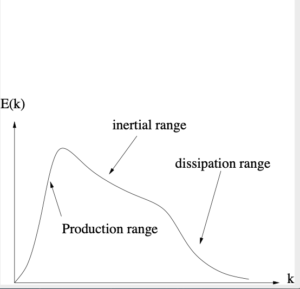
Various characteristic scales can be defined, but the most important is the Kolmogorov dissipation wavenumber, thus: $k_d=(\varepsilon /\nu_0^3)^{1/4}$, which gives the order of magnitude of the wavenumber at which the viscous effects begin to dominate. For the application of renormalized perturbation theory (which we will discuss in a later post), this phenomenology is important for assessment purposes. However, when we look at the later introduction of renormalization group theory, we have to consider this picture in rather more detail. We will do that in the next post.

[1] A. Berera, M. Salewski, and W. D. McComb. Eulerian Field-Theoretic Closure Formalisms for Fluid Turbulence. Phys. Rev. E, 87:013007-1-25, 2013.